The most useful result a ClickHouse performance audit produces is not a setting to change, and that focus is what separates a real ClickHouse performance audit from a settings sweep. It is a short list of queries that read far more than they return, with the reason for each one written down next to it. On ClickHouse 26.8 LTS that list is quicker to build than it was a year ago, because the server now tells you where the time went (EXPLAIN ANALYZE, since 26.7), lets you test a skip index before you build it (EXPLAIN WHATIF, since 26.6), and exposes which codec actually compressed each block (mergeTreeCodecBlockCounts(), new in 26.8).
This post is the working set of ClickHouse performance audit tips and tricks we use on 26.8, in the order we use them, with the real output from a lab run so you can compare shapes against your own cluster.
Everything below was run on ClickHouse 26.8.2.7 LTS (released 27 August 2026, supported to August 2027) on a deliberately small box: 2 vCPU, 7 GB RAM, a single MergeTree table of 40 million synthetic events in 16 parts across three monthly partitions. Absolute timings from a machine that size mean nothing for your estate, and no ClickHouse performance audit should quote them as targets.
The ratios, the plan shapes, and the columns we read from system.* are what transfer. If you want the 60-minute checklist version of a ClickHouse performance audit, we published that earlier as a complete ClickHouse performance audit in under 60 minutes; this piece is the layer underneath it, the tricks that decide whether the checklist finds anything.
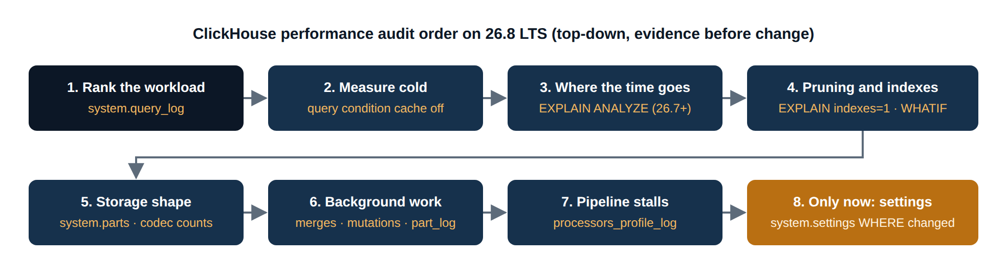
ClickHouse performance audit step one: rank the workload before you read a single setting
Start from system.query_log, not from system.settings. The question is not “is anything slow” but “which query shapes consume the cluster, and how much of what they read do they throw away”. Group by normalized_query_hash so that parameter values collapse into one row per shape, and add a column that most ClickHouse performance audit checklists skip: rows read per row returned. It is the single fastest indicator of a missing pruning path.
-- ClickHouse performance audit: which query shapes cost the most, and how wasteful each is
SELECT
    normalized_query_hash                        AS qhash,
    count()                                      AS runs,
    round(sum(query_duration_ms) / 1000, 1)      AS total_s,
    round(quantile(0.95)(query_duration_ms))     AS p95_ms,
    formatReadableSize(sum(read_bytes))          AS read,
    formatReadableSize(max(memory_usage))        AS peak_mem,
    round(sum(read_rows) / sum(result_rows))     AS rows_per_result_row,
    substring(any(query), 1, 60)                 AS sample
FROM system.query_log
WHERE type = 'QueryFinish'
  AND event_time >= now() - INTERVAL 1 HOUR
  AND is_initial_query
  AND query_kind = 'Select'
  AND query NOT LIKE '%system.%'
GROUP BY qhash
ORDER BY total_s DESC
LIMIT 5;
┌───────────────qhash─┬─runs─┬─total_s─┬─p95_ms─┬─read───────┬─peak_mem───┬─rows_per_result_row─┬─sample───────────────────────────────────────────────────────┐
1. │ 2039619392638216480 │ 3 │ 1.3 │ 447 │ 1.90 GiB │ 2.12 MiB │ 5000000 │ SELECT country, sum(bytes_out) FROM analytics.events_local W │
2. │ 9107957561281650861 │ 3 │ 1 │ 388 │ 380.52 MiB │ 324.93 MiB │ 475000 │ SELECT tenant_id, count() AS events, uniqExact(user_id) AS u │
3. │ 9090181284513977456 │ 1 │ 0.2 │ 156 │ 228.88 MiB │ 636.76 KiB │ 40000000 │ SELECT count(), min(event_date), max(event_date), uniq(tenan │
4. │ 1472193410336355370 │ 3 │ 0.2 │ 127 │ 310.18 MiB │ 229.80 KiB │ 13551787 │ SELECT count() FROM analytics.events_local WHERE user_id = 1 │
5. │ 3377994237059519770 │ 3 │ 0.2 │ 52 │ 112.61 MiB │ 3.61 MiB │ 412058 │ SELECT page_path, count() FROM analytics.events_local WHERE │
└─────────────────────┴──────┴─────────┴────────┴────────────┴────────────┴─────────────────────┴──────────────────────────────────────────────────────────────┘Two things stand out that a plain “slowest queries” list would hide from a ClickHouse performance audit. Row 2 is the only shape with a real memory footprint (325 MiB for uniqExact over a large key space), so it is the one that will hurt first when concurrency rises. Row 4 is a point lookup that reads 13.5 million rows per row it returns, which is the signature of a filter on a column that is not in the sort key. That row becomes the worked example for the rest of this ClickHouse performance audit.
Two small tricks here. On 26.6 and later, system.query_log also carries a client_agent column, which is worth grouping by if you suspect an AI coding assistant or a BI tool is generating the shapes you are looking at. And if you want engineers to audit their own queries without granting them system.query_log, 26.8 adds system.user_query_log, which shows each user only their own history.
Measure cold, or the query condition cache will flatter you
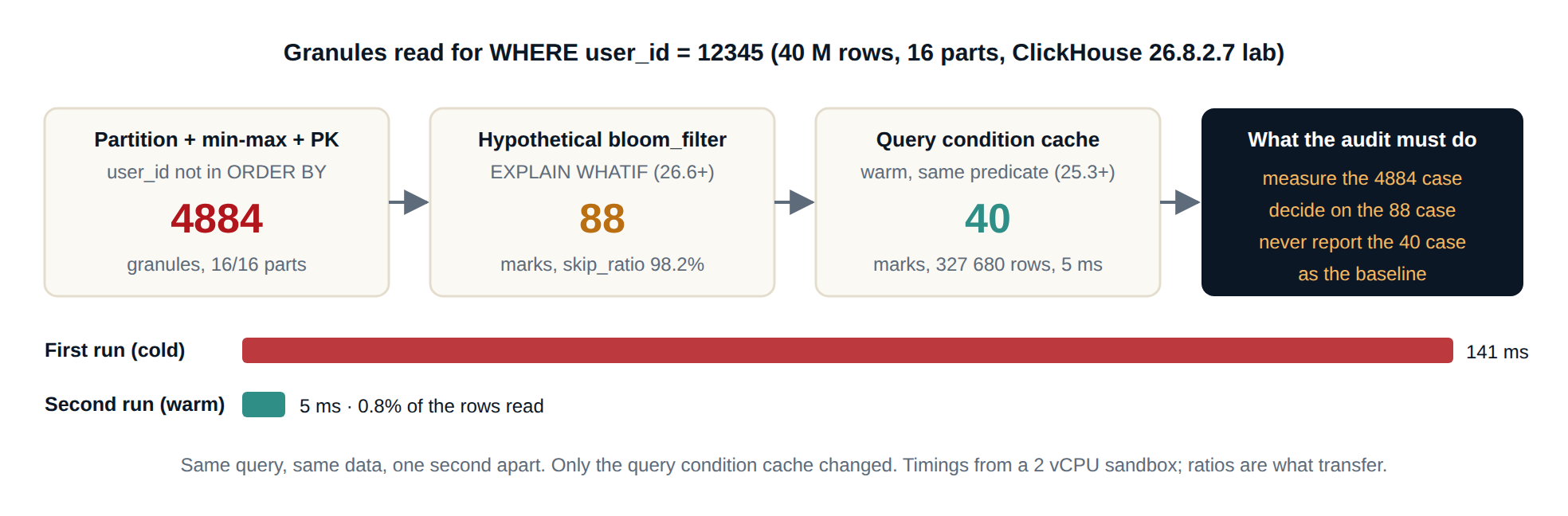
This is the trick that has changed the most since the 24.x line. Since 25.3, the query condition cache remembers, per part and per mark, which granules a predicate already proved to be empty. Re-run a query with the same WHERE clause and ClickHouse skips those granules without touching the primary index at all. That is excellent in production and a trap in a ClickHouse performance audit, because the second run of your test query is no longer measuring the table, it is measuring the cache.
Here is the same point lookup from row 4 above, five runs, taken straight from system.query_log with the relevant ProfileEvents keys pulled out:
SELECT
    event_time,
    query_duration_ms                                   AS ms,
    read_rows,
    ProfileEvents['QueryConditionCacheHits']            AS qcc_hits,
    ProfileEvents['QueryConditionCacheMisses']          AS qcc_misses,
    ProfileEvents['SelectedMarks']                      AS marks
FROM system.query_log
WHERE type = 'QueryFinish'
  AND query LIKE 'SELECT count() FROM analytics.events_local WHERE user_id = 12345%'
ORDER BY event_time_microseconds;
┌──────────event_time─┬──ms─┬─read_rows─┬─qcc_hits─┬─qcc_misses─┬─marks─┐
1. │ 2026-09-14 16:30:29 │ 141 │ 40000000 │ 0 │ 16 │ 4884 │
2. │ 2026-09-14 16:30:30 │ 5 │ 327680 │ 16 │ 0 │ 40 │
3. │ 2026-09-14 16:30:31 │ 4 │ 327680 │ 16 │ 0 │ 40 │
4. │ 2026-09-14 16:32:07 │ 6 │ 327680 │ 16 │ 0 │ 40 │
5. │ 2026-09-14 16:32:07 │ 5 │ 327680 │ 16 │ 0 │ 40 │
└─────────────────────┴─────┴───────────┴──────────┴────────────┴───────┘141 ms and 40 million rows on the first run; 5 ms and 327 680 rows on every run after it. Nothing about the table changed. If a ClickHouse performance audit report quotes the 5 ms number as the baseline, the recommendation that follows (add a skip index, change the sort key) will look pointless, and it will be wrong. Control for it explicitly, either per query or by clearing the cache before each cold measurement:
-- Option A: measure with the cache bypassed for this statement only
SELECT count()
FROM analytics.events_local
WHERE user_id = 12345
SETTINGS use_query_condition_cache = 0;

-- Option B: clear it once before a cold pass (safe; the cache rebuilds on demand)
SYSTEM DROP QUERY CONDITION CACHE;
The same discipline applies to the mark cache (ProfileEvents['MarkCacheHits']) and the OS page cache, which on Linux you can only reset with echo 3 > /proc/sys/vm/drop_caches on a box you are allowed to disturb. On a shared production replica, do not; take the cold-versus-warm delta from a query you are certain has not run in the last hour instead.
Let EXPLAIN ANALYZE say where the time went
Before 26.7, the honest way to attribute time inside a query was to join system.processors_profile_log by query_id and add up elapsed microseconds per processor. That still works and we still use it (see the pipeline section), but for the first pass EXPLAIN ANALYZE is faster to read. It runs the query, discards the result rows, and annotates every step of the logical plan with rows in and out, bytes, wall time, its share of the total, and the observed parallelism. This is the top query from the ranking above:
EXPLAIN ANALYZE
SELECT country, sum(bytes_out) AS egress
FROM analytics.events_local
WHERE referrer != ''
GROUP BY country;
Query summary:
Time: 468.25 ms (planning 32.97 ms · execution 435.29 ms)
Read: 40.00 million rows, 680.00 MB (91.89 million rows/s., 1.56 GB/s.)
Peak memory: 206.86 KiB
Output: country, sum(bytes_out)
Expression ((Project names + Projection))
│ I/O: rows 8 → 8 · 160 B → 160 B
│ time 3.76 us (0.0%) · parallelism 0.98/1
└──Aggregating
│ Keys: country
│ Aggregates: sum(bytes_out)
│ I/O: rows 32.00 million → 8 (0.00%) · 288.00 MB → 160 B
│ Stage (partial aggregation): time 127.01 ms (29.2%) · parallelism 1.11/2
│ Stage (final aggregation): time 23.14 us (0.0%) · parallelism 0.99/1
└──Expression (Before GROUP BY)
...
└──ReadFromMergeTree (analytics.events_local)
Read type: Default
Parts: 16 | Granules: 4884
Output: country, bytes_out
Prewhere filter
Prewhere filter column: referrer.size != 0
Indexes:
...
PrimaryKey
Condition: true
Parts: 16/16
Granules: 4884/4884
I/O: rows 0 → 32.00 million · 0 B → 288.00 MB
time 418.28 ms (96.1%) · parallelism 1.71/2This is the step of a ClickHouse performance audit that decides where effort goes. Read it bottom-up. 96.1% of the execution time is inside ReadFromMergeTree, so nothing you do to the aggregation will move this query; it is I/O bound on a full scan, and the only real levers are a sort key that includes the predicate, a projection, or reading fewer bytes per row (codecs).
Note two things the planner did on its own: it rewrote referrer != '' into a PREWHERE on referrer.size, reading the String’s size subcolumn instead of the string, and it dropped 8 million rows at read time so that the aggregation only saw 32 million. The parallelism figure, 1.71 of 2 threads, tells you the read pool kept both cores mostly busy. On a 64-core node a much lower ratio here is the first place to look for a max_threads or read-pool bottleneck.
One caveat on plan-annotated output: EXPLAIN ANALYZE executes the query in full, so run it with the same SETTINGS, the same cache state, and the same max_threads you are auditing, and never on a query whose cost you have not already bounded from system.query_log.
ClickHouse performance audit tip: read the fractions in EXPLAIN indexes = 1
EXPLAIN indexes = 1 has been in ClickHouse for years and is still the fastest way to see whether a predicate is being used for pruning or just for filtering. The ClickHouse performance audit trick is to read the three fractions, not the condition text. Here is the point lookup on a non-key column next to a lookup that uses both the partition key and the primary key:
EXPLAIN indexes = 1
SELECT count()
FROM analytics.events_local
WHERE user_id = 12345;
Aggregating
└──Filter ((WHERE + Change column names to column identifiers))
│ Filter column: user_id = 12345
└──ReadFromMergeTree (analytics.events_local)
Parts: 16 | Granules: 4884
Indexes:
Min-Max Condition: true Parts: 16/16 Granules: 4884/4884
Partition Condition: true Parts: 16/16 Granules: 4884/4884
PrimaryKey Condition: true Parts: 16/16 Granules: 4884/4884Condition: true at every level means “I could not use this predicate here at all”. Compare it with the shape you want to see:
EXPLAIN indexes = 1
SELECT count()
FROM analytics.events_local
WHERE tenant_id = 42
  AND event_date BETWEEN '2026-07-01' AND '2026-07-31';
AggregatingProjection
├──ReadFromMergeTree (analytics.events_local)
│ Parts: 6 | Granules: 10
│ Prewhere filter column: tenant_id = 42 AND event_date <= '2026-07-31' AND event_date >= '2026-07-01'
│ Indexes:
│ Min-Max Keys: event_date Parts: 6/16 Granules: 1892/4884
│ Partition Keys: toYYYYMM(event_date) Parts: 6/6 Granules: 1892/1892
│ PrimaryKey Keys: tenant_id, event_date Parts: 6/6 Granules: 10/1892
│ Search Algorithm: binary search
└──ReadFromPreparedSource (_exact_count_projection)Ten granules out of 4 884 is the shape a ClickHouse performance audit wants to see, and the count itself is answered from the implicit exact-count projection rather than by scanning them. When a ClickHouse performance audit covers a customer’s top twenty query shapes, put these fractions in a table: shape, granules selected over granules total at the primary-key level. Anything above roughly 20% with a selective predicate is a candidate for the next section; anything at 100% with Condition: true is a sort-key conversation, not an index conversation.
Try the index before you build it (EXPLAIN WHATIF)
Adding a data-skipping index to a multi-terabyte table means a MATERIALIZE INDEX mutation that rewrites index files for every part, and if the index turns out not to help you have spent the I/O for nothing. Since 26.6 you can define the index hypothetically in your session and ask the planner what it would have skipped:
CREATE HYPOTHETICAL INDEX idx_user_bf
    ON analytics.events_local (user_id)
    TYPE bloom_filter(0.01)
    GRANULARITY 4;

EXPLAIN WHATIF
SELECT count()
FROM analytics.events_local
WHERE user_id = 12345;
Baseline (after PK + partition + existing indexes):
table: analytics.events_local
parts: 16
marks: 4884
est_bytes: 1.06 GiB
With idx_user_bf (bloom_filter, hypothetical):
status: applicable
marks: 88
est_bytes: 19.48 MiB
skip_ratio: 98.2%
Estimation:
source: empirical
empirical_status: ok
sampled_parts: 16 / 16
sampled_marks: 4884 / 8720
elapsed_us: 2127998A 98.2% skip ratio on a bloom filter with granularity 4 is a build decision made in two seconds instead of a mutation on a production table. Three practical notes from using it in a ClickHouse performance audit.
The hypothetical index lives in the session that created it (it shows up in system.hypothetical_indexes, and a fresh clickhouse-client will report “No hypothetical indexes defined”), so run the definition and the EXPLAIN in the same connection. The empirical source means the planner sampled real marks rather than estimating from statistics, which is what you want for a decision, at the price of the two-second read. And a positive result still needs the production caveat: build the index with ALTER TABLE ... ADD INDEX first, then MATERIALIZE INDEX partition by partition during a quiet window, checking system.mutations between partitions, on a replica whose backup you have restored recently.
ClickHouse performance audit of the storage layer: parts, per-column ratios, and which codec really ran
Query-side fixes stop paying off once the bytes per row are the problem, so the storage layer gets its own pass in every ClickHouse performance audit we run. Three queries cover it. First, part count and compression per partition from system.parts, which is where “too many parts” shows up long before it becomes error 252:
SELECT
    partition,
    count()                                                              AS parts,
    sum(rows)                                                            AS rows,
    formatReadableSize(sum(data_compressed_bytes))                       AS on_disk,
    round(sum(data_uncompressed_bytes) / sum(data_compressed_bytes), 2)  AS ratio,
    formatReadableSize(sum(primary_key_bytes_in_memory))                 AS pk_in_ram
FROM system.parts
WHERE database = 'analytics' AND table = 'events_local' AND active
GROUP BY partition
ORDER BY partition;
┌─partition─┬─parts─┬─────rows─┬─on_disk────┬─ratio─┬─pk_in_ram─┐
1. │ 202606 │ 5 │ 15000000 │ 405.21 MiB │ 2.57 │ 10.18 KiB │
2. │ 202607 │ 6 │ 15500000 │ 418.72 MiB │ 2.57 │ 10.34 KiB │
3. │ 202608 │ 5 │ 9500000 │ 256.64 MiB │ 2.57 │ 6.03 KiB │
└───────────┴───────┴──────────┴────────────┴───────┴───────────┘Second, the same ratio per column from system.parts_columns. A table-level ratio of 2.57 hides the fact that four columns are doing almost all the damage:
SELECT
    column,
    any(type)                                                                        AS type,
    formatReadableSize(sum(column_data_compressed_bytes))                            AS on_disk,
    round(sum(column_data_uncompressed_bytes) / sum(column_data_compressed_bytes), 1) AS ratio
FROM system.parts_columns
WHERE database = 'analytics' AND table = 'events_local' AND active
GROUP BY column
ORDER BY sum(column_data_compressed_bytes) DESC;
┌─column──────┬─type───────────────────┬─on_disk────┬─ratio─┐
1. │ page_path │ String │ 229.83 MiB │ 2.6 │
2. │ referrer │ String │ 200.06 MiB │ 4.8 │
3. │ user_id │ UInt64 │ 188.27 MiB │ 1.6 │
4. │ bytes_out │ UInt64 │ 160.66 MiB │ 1.9 │
5. │ event_time │ DateTime │ 152.79 MiB │ 1 │
6. │ duration_ms │ UInt32 │ 111.33 MiB │ 1.4 │
7. │ country │ LowCardinality(String) │ 32.35 MiB │ 1.2 │
8. │ event_type │ LowCardinality(String) │ 1.55 MiB │ 24.6 │
9. │ tenant_id │ UInt32 │ 728.62 KiB │ 214 │
10. │ event_date │ Date │ 536.31 KiB │ 145.3 │
└─────────────┴────────────────────────┴────────────┴───────┘An event_time column at a ratio of 1.0 is a codec problem, not a data problem. Third, and new in 26.8, mergeTreeCodecBlockCounts() tells you which codec was actually applied per block, which matters once you start using the experimental adaptive codec selection (enable_adaptive_codec_selection, a MergeTree setting, off by default in 26.8) and need to prove what it chose:
SELECT column, sumMap(codec_block_counts) AS blocks
FROM mergeTreeCodecBlockCounts('analytics', 'events_local')
WHERE column IN ('duration_ms', 'bytes_out', 'event_time')
GROUP BY column;
┌─column──────┬─blocks───────┐
1. │ duration_ms │ {'LZ4':2438} │
2. │ event_time │ {'LZ4':2438} │
3. │ bytes_out │ {'LZ4':4873} │
└─────────────┴──────────────┘Plain LZ4 on every block, which is the default and explains the ratios a ClickHouse performance audit sees on most untouched tables. We copied the August partition into a sibling table with explicit codecs to see what a targeted change is worth on this data:
ALTER TABLE analytics.events_codec MODIFY COLUMN event_time  DateTime CODEC(DoubleDelta, ZSTD(1));
ALTER TABLE analytics.events_codec MODIFY COLUMN duration_ms UInt32   CODEC(T64, ZSTD(1));
ALTER TABLE analytics.events_codec MODIFY COLUMN bytes_out   UInt64   CODEC(T64, ZSTD(1));
ALTER TABLE analytics.events_codec MODIFY COLUMN user_id UInt64 CODEC(ZSTD(1));| Column (partition 202608) | Default LZ4 | Explicit codec | Change on disk |
|---|---|---|---|
event_time | 36.36 MiB, ratio 1.0 | 24.07 MiB, ratio 1.5 | 34% smaller |
duration_ms | 26.51 MiB, ratio 1.4 | 13.55 MiB, ratio 2.7 | 49% smaller |
bytes_out | 38.24 MiB, ratio 1.9 | 20.35 MiB, ratio 3.5 | 47% smaller |
user_id | 44.82 MiB, ratio 1.6 | 31.77 MiB, ratio 2.3 | 29% smaller |
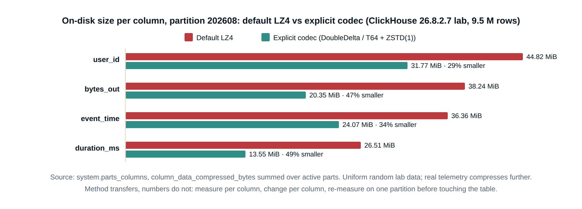
system.parts_columns on partition 202608.Be careful with what this table proves. The lab data is uniformly random inside each column, which is close to the worst case for every codec; real telemetry with monotonic timestamps and skewed values compresses far better than this, and the relative ordering of codecs can change. Treat it as a demonstration of the method (measure per column, change per column, measure again on one partition) rather than as a recommendation for those four codecs.
Look at the background work before blaming the foreground
A cluster that is slow at 09:00 and fine at 11:00 is usually paying for merges or a mutation, not for a bad query, and a ClickHouse performance audit that skips the background layer will misattribute it. Three system tables answer it in one pass: system.merges for what is running now, system.mutations for what is stuck, and system.part_log for the write pattern over the last hour.
SELECT database, table, count() AS running_merges,
       round(max(elapsed)) AS longest_s, round(max(progress) * 100) AS max_progress_pct,
       formatReadableSize(sum(total_size_bytes_compressed)) AS bytes_in_flight
FROM system.merges
GROUP BY database, table;

SELECT database, table, count() AS pending_mutations, min(create_time) AS oldest,
       anyIf(latest_fail_reason, latest_fail_reason != '') AS fail_reason
FROM system.mutations
WHERE NOT is_done
GROUP BY database, table;

SELECT event_type, count() AS n, round(avg(duration_ms)) AS avg_ms,
       formatReadableSize(sum(size_in_bytes)) AS bytes, sum(rows) AS rows
FROM system.part_log
WHERE event_time >= now() - INTERVAL 1 HOUR AND table = 'events_local'
GROUP BY event_type;
┌─event_type──────┬──n─┬─avg_ms─┬─bytes──────┬─────rows─┐
1. │ NewPart │ 41 │ 516 │ 1.06 GiB │ 40000000 │
2. │ MergeParts │ 5 │ 4221 │ 838.85 MiB │ 31046048 │
3. │ MergePartsStart │ 5 │ 0 │ 0.00 B │ 0 │
└─────────────────┴────┴────────┴────────────┴──────────┘The lab was idle for the first two queries (no output), which is what a healthy hour looks like in a ClickHouse performance audit. The part_log ratio is the number to keep: 41 parts written, 31 million of the 40 million rows re-read by merges within the hour. On a cluster with small, frequent inserts that ratio goes above 3x, and the fix is on the insert side (batch size, async_insert) rather than in the merge scheduler. If pending_mutations is non-zero with a fail_reason, stop the ClickHouse performance audit and deal with it; a failed mutation blocks every mutation queued behind it.
ClickHouse performance audit: find pipeline stalls with processors_profile_log
When EXPLAIN ANALYZE says the time is in aggregation rather than in the read, the next ClickHouse performance audit question is whether the aggregation was working or waiting. system.processors_profile_log (on by default via log_processors_profiles = 1) records per processor how long it was busy, how long it waited for input, and how long it waited for its output to be consumed. This is the uniqExact query from row 2 of the ranking:
SELECT
    name                                       AS processor,
    count()                                    AS instances,
    round(sum(elapsed_us) / 1000)              AS busy_ms,
    round(sum(input_wait_elapsed_us) / 1000)   AS wait_in_ms,
    round(sum(output_wait_elapsed_us) / 1000)  AS wait_out_ms,
    sum(input_rows)                            AS in_rows,
    sum(output_rows)                           AS out_rows
FROM system.processors_profile_log
WHERE query_id = '${QUERY_ID}'
GROUP BY processor
ORDER BY busy_ms DESC
LIMIT 8;
┌─processor──────────────────────────────────────────┬─instances─┬─busy_ms─┬─wait_in_ms─┬─wait_out_ms─┬──in_rows─┬─out_rows─┐
1. │ AggregatingTransform │ 2 │ 301 │ 92 │ 76 │ 9500400 │ 400 │
2. │ ConvertingAggregatedToChunksWithMergingSource │ 2 │ 151 │ 0 │ 5 │ 0 │ 400 │
3. │ MergeTreeSelect(pool: ReadPool, algorithm: Thread) │ 2 │ 85 │ 0 │ 302 │ 0 │ 9500000 │
4. │ ExpressionTransform │ 7 │ 1 │ 850 │ 605 │ 19000420 │ 19000420 │
5. │ PartialSortingTransform │ 2 │ 1 │ 552 │ 1 │ 400 │ 400 │
6. │ MergeSortingTransform │ 2 │ 1 │ 554 │ 0 │ 400 │ 40 │
7. │ MergingSortedTransform │ 1 │ 0 │ 277 │ 0 │ 40 │ 20 │
8. │ ConvertingAggregatedToChunksTransform │ 1 │ 0 │ 6 │ 74 │ 400 │ 400 │
└────────────────────────────────────────────────────┴───────────┴─────────┴────────────┴─────────────┴──────────┴──────────┘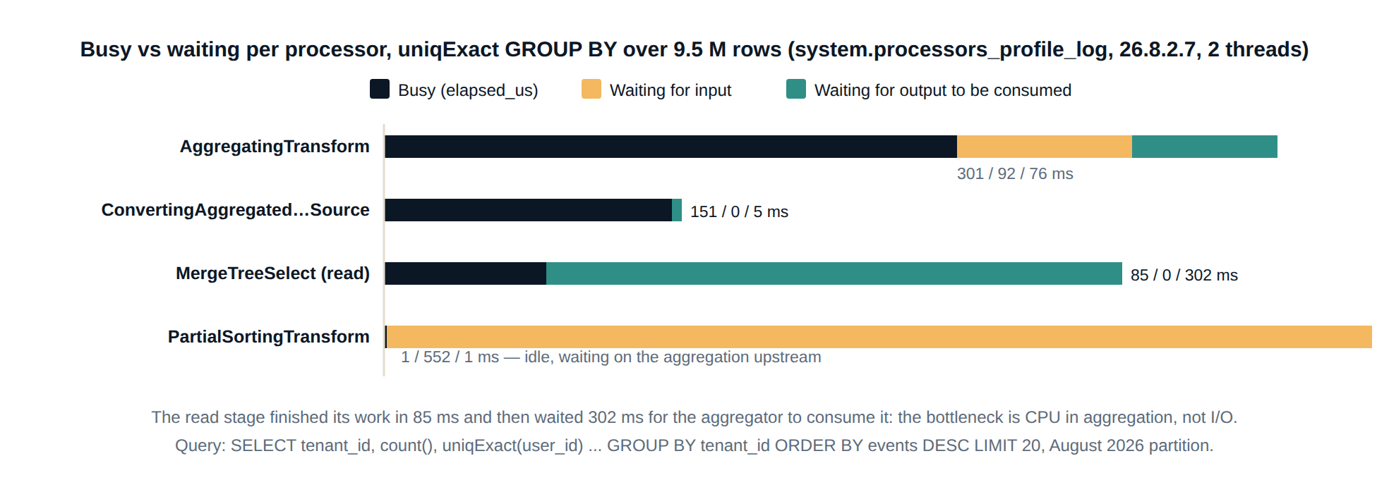
processors_profile_log rows as a busy-versus-waiting breakdown. The read stage is idle for most of the query; the aggregator is the one working.Read the third row against the first. The read stage was busy for 85 ms and spent 302 ms waiting for someone to take its output; the aggregating stage was the one doing the work, 301 ms busy for 9.5 million input rows. That is a CPU-bound aggregation on a two-thread box, and the honest recommendation is more cores or fewer distinct keys, not a storage change.
The 26.8 adaptive aggregator (enable_adaptive_aggregator, on by default) chooses between merging and splitting strategies per query, and the packed single-String-key hash table (enable_packed_string_keys_in_aggregation, also on by default) shrinks the cell size; both show up here as lower busy_ms in AggregatingTransform when you compare the same query on 26.3 and 26.8, which is the right way to measure an upgrade.
Only now, settings: what a ClickHouse performance audit should verify on 26.8
Settings come last because most of the ones that matter on 26.8 are already on, and the ClickHouse performance audit’s job is to confirm they have not been switched off by a profile, a client, or a leftover from a 24.x runbook. The two-line check is SELECT name, value, default FROM system.settings WHERE changed, and the same for system.merge_tree_settings. On a fresh 26.8.2.7 the defaults that a ClickHouse performance audit should know about look like this:
| Audit signal | Source | Since | What to check |
|---|---|---|---|
| Query shapes and waste ratio | system.query_log | always | read_rows / result_rows per normalized_query_hash; client_agent from 26.6 |
| Warm-cache distortion | ProfileEvents | 25.3 | QueryConditionCacheHits non-zero means the run was not cold; use_query_condition_cache = 1 by default |
| Time per plan step | EXPLAIN ANALYZE | 26.7 | Percentage in ReadFromMergeTree versus Aggregating; observed parallelism versus max_threads |
| Pruning effectiveness | EXPLAIN indexes = 1 | always | PrimaryKey granule fraction; Condition: true means the predicate is not usable |
| Skip-index value before build | EXPLAIN WHATIF | 26.6 | skip_ratio with source: empirical; session-scoped definition |
| Codec actually applied | mergeTreeCodecBlockCounts() | 26.8 | Per-block codec map; pairs with enable_adaptive_codec_selection (experimental, off) |
| Join planning inputs | system.settings | 26.2 / 26.8 | use_statistics = 1, materialize_statistics_on_insert = 1, auto_statistics_types = basic, uniq_v2; join_algorithm default list now includes ie_join |
| Aggregation strategy | system.settings | 26.8 | enable_adaptive_aggregator = 1, enable_packed_string_keys_in_aggregation = 1; compare AggregatingTransform busy time across versions |
| Background pressure | system.part_log | always | Rows merged per hour divided by rows inserted per hour; failed mutations block the queue |
A short note on the statistics row, because it changes how you read join plans. Column statistics have been built during background merges since 26.2; 26.8 also materialises them on insert for tables below materialize_statistics_on_insert_max_table_size (25 GiB by default), so a freshly loaded dimension table now carries cardinality estimates immediately. If a join picks a surprising algorithm on 26.8, check whether the estate has use_statistics = 0 in a profile from before the feature stabilised; several of the clusters we support did.
Key takeaways from a ClickHouse performance audit on 26.8
- Start every ClickHouse performance audit by ranking query shapes by total time and by rows read per row returned from
system.query_logbefore you look at any setting; the second number finds missing pruning paths faster than latency does. - Control for the query condition cache (25.3+) in every cold measurement. In the lab it turned a 141 ms, 40-million-row scan into a 5 ms, 327 680-row read with no schema change, which is exactly the kind of number a ClickHouse performance audit must not report as a baseline.
- Use
EXPLAIN ANALYZE(26.7+) in a ClickHouse performance audit to attribute time to plan steps andEXPLAIN indexes = 1to read granule fractions; a 96% share inReadFromMergeTreemeans the fix is in the sort key, projection, or codec, never in the aggregation. - Test skip indexes with
EXPLAIN WHATIF(26.6+) before the ClickHouse performance audit recommends a build, in the same session that defined the hypothetical index; a 98% skip ratio measured in two seconds is worth more than a mutation started on faith. - Audit compression per column in every ClickHouse performance audit and, on 26.8, per block with
mergeTreeCodecBlockCounts(); a numeric or time column at ratio 1.0 on LZ4 is a codec decision waiting to be made, and one partition is enough to measure it. - In a ClickHouse performance audit, read merges, mutations, and
part_logbefore blaming foreground queries, and readprocessors_profile_logto tell busy from waiting. Then, and only then, diffsystem.settings WHERE changedagainst the 26.8 defaults.
FAQ
Does EXPLAIN ANALYZE run the query on ClickHouse 26.8?
Yes, which is why a ClickHouse performance audit should run it deliberately rather than casually. It executes every phase, discards the result rows, and annotates the plan with measured time, rows, bytes, and parallelism per step. Bound the query’s cost from system.query_log first and run it with the settings and cache state the ClickHouse performance audit is measuring.
Why is my second test run so much faster than the first on 26.8?
This is the most common false positive in a ClickHouse performance audit on 25.3 and later. Most often the query condition cache has recorded which granules the predicate already ruled out. Check ProfileEvents['QueryConditionCacheHits'] in system.query_log; if it is non-zero, repeat the measurement with use_query_condition_cache = 0 or after SYSTEM DROP QUERY CONDITION CACHE.
Is EXPLAIN WHATIF safe to run on a production table?
The hypothetical index is session-scoped metadata and writes nothing to disk. With empirical estimation it does read a sample of marks, which in the lab cost about two seconds on 40 million rows, so a ClickHouse performance audit should run it on a replica or in a quiet window on very large tables.
Which ClickHouse versions do these ClickHouse performance audit tips apply to?
The system.query_log, system.parts, EXPLAIN indexes = 1, and processors_profile_log techniques work on any supported release. EXPLAIN WHATIF and client_agent need 26.6, EXPLAIN ANALYZE needs 26.7, and mergeTreeCodecBlockCounts(), statistics on insert, and system.user_query_log need 26.8 LTS. Confirm your exact build with SELECT version() before relying on any of them.
The standing caveat applies to every command above. Test on staging with your own workload before touching production, keep a verified backup and a rehearsed restore, and treat the DR replica as part of the estate the ClickHouse performance audit covers. If you would rather have a second pair of eyes on the findings, or a ClickHouse performance audit run against a Severity 1 response commitment of fifteen minutes, that is what the ChistaDATA ClickHouse support team does every week; the contact page is the fastest way to start.
Sources: ClickHouse 26.8 release call, ClickHouse 26.7 release notes, ClickHouse 26.6 release call, ClickHouse EXPLAIN reference, ClickHouse release and support calendar. Lab: ClickHouse 26.8.2.7 LTS, 2 vCPU / 7 GB, 40 million synthetic rows, single node.
Running ClickHouse in production? ChistaDATA provides ClickHouse consulting for architecture, performance and migrations, and 24×7 ClickHouse support with a 15-minute S1 response. For day-to-day operations see ClickHouse DBA services and ClickHouse managed services.
