ChistaDATA · ClickHouse internals, measured on 1,000,000,000 rows · re-checked on 26.8 LTS
Why ClickHouse is so fast is best answered with a number: on a two-core machine with 7 GB of memory, it averaged a column across 1,000,000,000 rows in 1.06 seconds on ClickHouse 26.7, roughly 940 million rows per second, and answered a per-tenant question over the same billion rows in 8 milliseconds by reading 7 granules out of 122,127. Neither result needed a cluster, a cache or a ClickHouse performance tuning pass. Both follow from seven design choices that run through every layer of the engine, and together they are why ClickHouse is so fast at any scale we have measured.
Re-run on ClickHouse 26.8.11.7 LTS in September 2026, the same query took 0.74 seconds, 1.34 billion rows per second, and the section that follows the introduction puts both runs side by side.
This article measures each of those seven choices on ClickHouse 26.7 against a billion-row events table we generated for the purpose, with the relevant setting switched off wherever the engine allows it so that the contribution is isolated rather than asserted. It also places our lab numbers next to the published figures from the largest ClickHouse deployments in the world, clearly marked as theirs, because the point of understanding why ClickHouse is so fast is knowing how far the same mechanisms carry.
All lab figures: ClickHouse 26.7.2.1, 2 vCPU / 7 GB / local NVMe-class disk, median of three runs with use_query_condition_cache = 0 unless stated. The table is larger than memory, so these are ClickHouse performance numbers from disk, not warm-cache numbers. Re-run: ClickHouse 26.8.11.7 LTS on 26 September 2026, same machine class and generator, query condition cache off, caches dropped before every first run.
Re-checked on 26.8 LTS · September 2026
We re-ran the lab on ClickHouse 26.8 LTS and read the 26.9 notes. Here is what held and what moved
The numbers in the body were taken on ClickHouse 26.7.2.1. Since then 26.8 became the LTS line (announced 10 September 2026: 98 new features, 128 performance optimisations, 556 bug fixes) and 26.9 landed on 24 September (56, 135 and 464). So on 26 September we did the boring but necessary thing: same generator, same 1,000,000,000 rows, same 2 vCPU / 7 GB / NVMe-class box, ClickHouse 26.8.11.7 LTS, query condition cache off, mark and uncompressed caches dropped before every first run, server-side medians of three from system.query_log.
Then we went through every sentence in the body that names a version, a default or a feature and checked it against the binary’s system.settings and system.merge_tree_settings, and against the 26.9 release call.
Short version: the seven reasons why ClickHouse is so fast are the same seven. None of them was replaced, and nothing in 26.8 or 26.9 makes any of them less true. What changed is the constants. Every full-scan query on this table got faster on the same hardware, which is the plainest evidence for why ClickHouse is so fast that we can offer, automatic column statistics now prune parts without any DDL from us, and lazy materialization is a real eighth reason why ClickHouse is so fast on ORDER BY ... LIMIT that the original article did not measure.
We kept the 26.7 figures in the body so the plans, tables and prose stay consistent with each other; the table below is the side-by-side.
One thing worth admitting up front: the first 26.8 load ran out of disk at about 650 million rows, because outdated parts from the background merges had not been cleaned up yet and the box only has 30 GB free. We set old_parts_lifetime to 30 seconds on the table, dropped the one partition that had received a partial batch, reloaded it from the generator and checked that the count was exactly 1,000,000,000 before measuring anything. If you reproduce this on a small machine, budget disk for roughly twice the final table size during the load; none of it changes why ClickHouse is so fast, but it will change whether you get to find out.
| Query on the 1,000,000,000-row table | 26.7.2.1 (body) | 26.8.11.7 LTS (re-run) | Note |
|---|---|---|---|
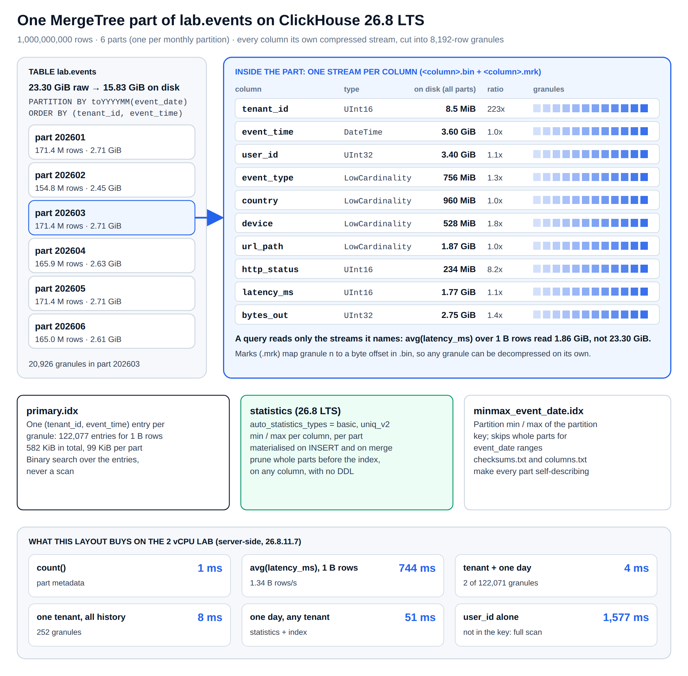
avg(latency_ms), count() | 1,064 ms · 940 M rows/s | 744 ms · 1.34 B rows/s | one 2-byte column, 1.86 GiB read |
count() WHERE http_status >= 500 | 1,021 ms | 709 ms | 1.41 B rows/s |
sum(bytes_out) | 3,066 ms | 1,557 ms | 4-byte column, 3.73 GiB |
GROUP BY event_type | 3,127 ms | 2,591 ms | adaptive aggregator is on by default |
uniqCombined(user_id) | 3,487 ms | 2,294 ms | runs varied 2.2 to 2.6 s; median shown |
GROUP BY tenant_id with sum(bytes_out) | 4,570 ms | 3,683 ms | two columns, 5.59 GiB |
| one tenant, one day (sort-key prefix) | 8 ms · 7 granules | 4 ms · 2 of 122,071 granules | statistics drop 5 of 6 parts, then binary search |
| one tenant, all history (2.06 M rows) | 31 ms | 8 ms · 252 granules | |
| one day, any tenant (second key column) | 96 ms | 51 ms · 1,186 granules | statistics first, generic exclusion search second |
user_id = 4200042 alone (not in the key) | 2,875 ms | 1,577 ms | still a full scan of one 3.40 GiB column |
| the same predicate, second run, query condition cache on | 19 ms (100x) | 12 ms (135x) · 90 granules | on by default since 25.3 |
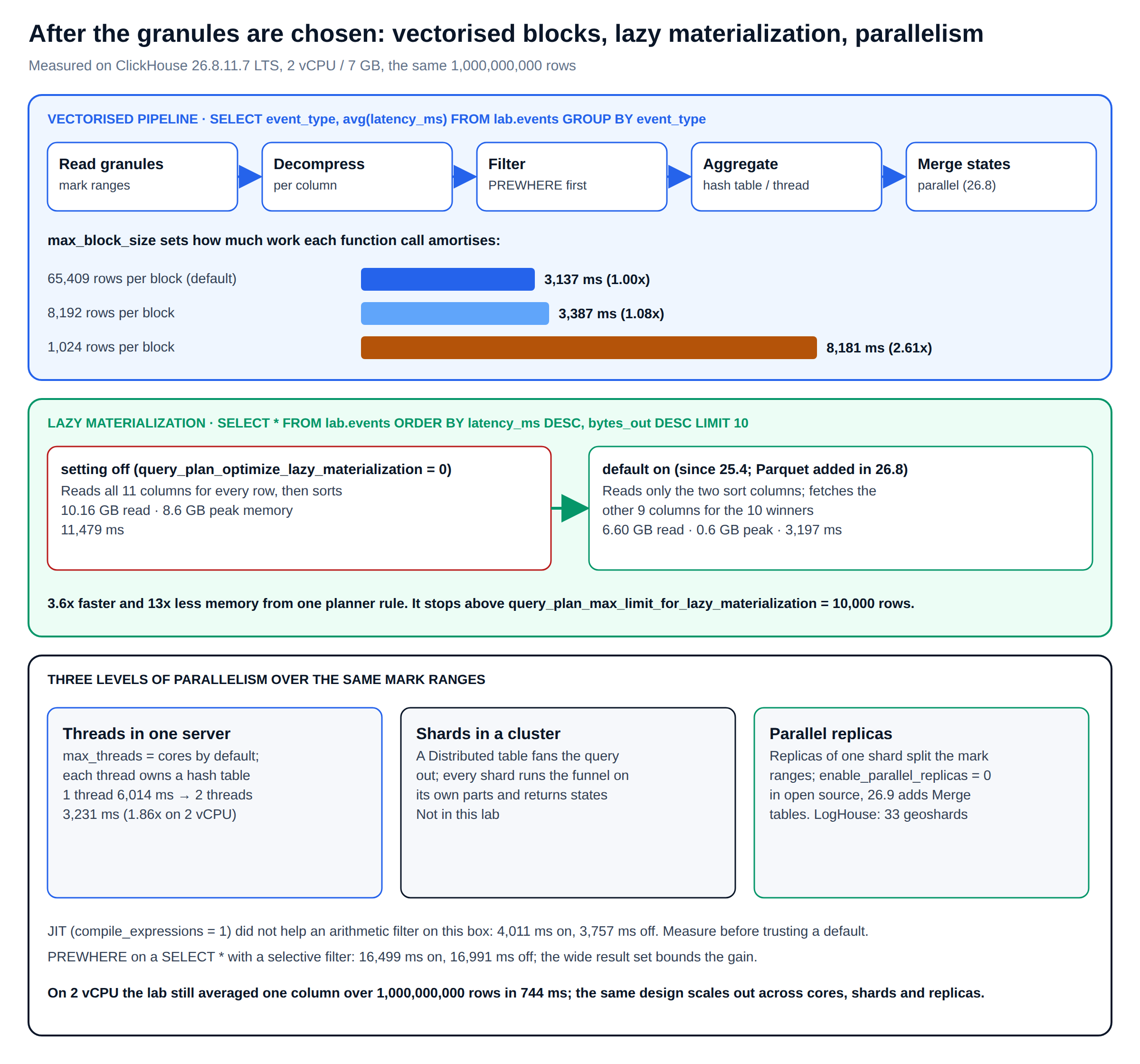
SELECT * ... ORDER BY latency_ms DESC, bytes_out DESC LIMIT 10 | not measured | 3,197 ms on · 11,479 ms off | lazy materialization, default on; peak memory 0.6 GB against 8.6 GB |
max_threads = 1 to 2, GROUP BY event_type | 8,640 to 4,457 ms (1.94x) | 6,014 to 3,231 ms (1.86x) | slightly less than last time; two cores is a small sample |
GROUP BY country, device (composite LowCardinality) | 25 s | 18.3 s | better, still the slowest shape on this box; turning the adaptive aggregator off made no difference (18.6 s) |
quantile(0.95)(latency_ms) by country, device | 27 s | 21.7 s | |
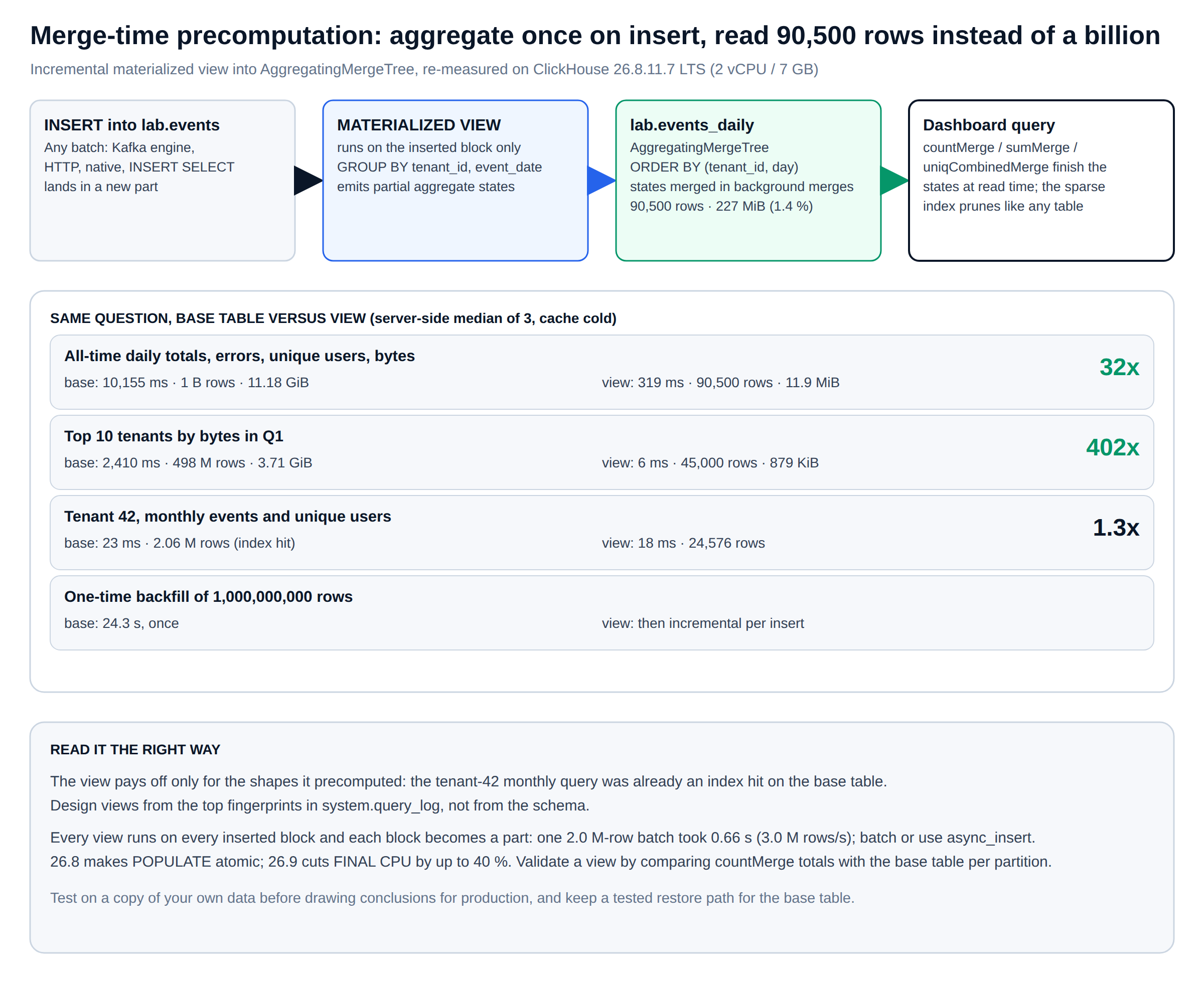
| daily view versus base table (Q1 top-10 tenants) | 4,455 to 271 ms (16x) | 2,410 to 6 ms (402x) | view: 90,500 rows, 227 MiB, 24.3 s backfill |
| tuned codecs on the full table | 99.5 M-row slice: 887 MiB (2.68x) | 8.70 GiB against 15.83 GiB with LZ4 (2.68x) | but avg(latency_ms) went from 744 to 1,308 ms: ZSTD and T64 decode costs CPU this box does not have |
Table 0. The 26.7 lab against the 26.8 LTS re-run, or why ClickHouse is so fast on the same box a release later. Same generator, same machine class, server-side medians of three runs from system.query_log, first runs with caches cold.
What we checked against 26.8 and 26.9, what we corrected, and what it says about why ClickHouse is so fast
Statistics first. The body says the 26.7 build maintains part-level column statistics automatically, and that is now stronger than we wrote: on 26.8 the binary reports materialize_statistics_on_insert = 1 (for tables up to 25 GiB), use_statistics_for_part_pruning = 1 and auto_statistics_types = basic, uniq_v2. That is why ClickHouse is so fast on the one-tenant-one-day query now, touching 2 granules instead of 7, and why the second-key-column query halved. The 26.9 release call goes further and answers min, max and count straight from statistics (8 to 24 ms became 2 ms in their example). We did not re-measure that one.
Lazy materialization next. It arrived in 25.4 and is on by default; 26.8 extends it to Parquet on object storage and to local files (the release post’s S3 example drops from about 6.7 GB read to 1.5 GB). On our billion rows it took a SELECT * top-10 from 11,479 ms to 3,197 ms and cut peak memory from 8.6 GB to 0.6 GB; on a wide top-N this is now a large part of why ClickHouse is so fast. The planner stops applying it above query_plan_max_limit_for_lazy_materialization = 10000 rows, which is worth knowing before you paginate with large offsets.
Query condition cache. The body said “the 26.x line adds” it. That was sloppy: it shipped in 25.3 and has been on by default since; 26.8 also applies it to TopK queries (use_query_condition_cache_for_top_k = 1). We corrected the sentence. The advice stands, and it matters for anyone measuring why ClickHouse is so fast: benchmark with it off, run production with it on, and do not report a warm second run as if it were the first.
Aggregation and joins. 26.8 ships an adaptive parallel GROUP BY (enable_adaptive_aggregator = 1), packed string keys, a multi-threaded final merge and, per the changelog, a 2.4x faster DISTINCT on sorted prefixes; joins get IEJoin for inequality conditions, a parallel_full_sorting_merge algorithm and statistics-driven planning that ClickHouse measured at 29 % on TPC-H. 26.9 adds a faster LEFT SEMI JOIN (0.50 s to 0.37 s in the release call).
The composite LowCardinality GROUP BY that we flagged as a limit improved from 25 s to 18.3 s, which is less than we hoped for from the packed keys; it remains the slowest shape in this article, a reminder that why ClickHouse is so fast is always a per-query-shape question, and the limits section still applies.
Parallel replicas and merges. enable_parallel_replicas = 0 is still the open-source default on 26.8.11.7, so level-3 parallelism, the cluster half of why ClickHouse is so fast, stays opt-in exactly as the body says; 26.9 extends parallel replicas to Merge tables with distributed aggregation. Merges now choose codecs adaptively (26.8), and 26.9’s k-way merge is 7 to 8 % faster on multi-column keys with up to 40 % less CPU for FINAL, which matters for the ReplacingMergeTree patterns in our archival work more than for this table.
Two smaller corrections, and one non-result. The skip-index table said text supersedes tokenbf_v1 and ngrambf_v1; the accurate statement is that the 26.x documentation marks those two as deprecated and lists text as the current full-text type, so the table now says that. And on JIT: compile_expressions = 1 is the default, but on this two-core box it made an arithmetic filter slightly slower (4,011 ms on, 3,757 ms off). We are not going to draw a conclusion from one query on two cores except the one the settings table already draws, which is to measure rather than assume, even when the question is why ClickHouse is so fast rather than whether.
The codec result is the one that surprised us. Tuned per-column codecs shrank the full table from 15.83 GiB to 8.70 GiB, which on a disk-bound box we expected to make scans faster. It made them slower, because ZSTD and T64 decoding is CPU work and this machine has two cores to give.
On the 16- and 32-core nodes we run for customers the trade usually goes the other way, but that is a claim about other hardware, so treat the storage number as measured and the speed number as something to test on your own core count. The engine is the same either way; why ClickHouse is so fast per byte depends on whether the box has CPU to spare for decoding.
Checked on 26 September 2026 against ClickHouse release 26.8, the 26.9 release call, the 2026 changelog, GitHub releases (v26.9.2.8-stable and v26.8.11.7-lts, 22 September 2026), the MergeTree documentation and the 25.3 and 25.4 release posts. Settings were read from the 26.8.11.7 binary itself.
Scale
The scale at which why ClickHouse is so fast actually matters
A billion rows is a useful laboratory size because it is large enough to exceed memory and small enough to rebuild in eight minutes. It is not large by ClickHouse standards, and why ClickHouse is so fast at a billion rows is only interesting because the same answer holds at a quadrillion. The published production figures below are the reference points we keep in mind when we design a cluster; they are the vendors’ and operators’ own numbers, cited to source, not ours.
| Deployment | Published scale | Source |
|---|---|---|
| Cloudflare analytics | A single query covering 96 trillion events in one hour, and 1.61 quadrillion events over a full day, returning in under two seconds; open-source ClickHouse in production for close to ten years across more than 300 data centres | ClickHouse blog, Cloudflare |
| ClickHouse LogHouse (internal observability) | 1.59 × 10¹⁵ rows; 431 PiB uncompressed stored as 27 PiB on disk, a 16x compression ratio; peak ingest of 190 million rows per second and 80 GiB/s across about 5,800 inserts per second; 33 geoshards on three clouds | ClickHouse blog, LogHouse |
| ClickBench (independent, reproducible) | 99,997,497-row web-analytics table, 43 queries covering full scans, filtered scans, index lookups and the main relational operators; cold and hot runs published per engine | ClickBench on GitHub |
| This article | 1,000,000,000 rows, 11 columns, 15.84 GiB compressed, 2 vCPU, every number reproducible from the appendix | Below |
Table 1. Published scale references beside the lab, the context in which ClickHouse performance claims should be read. Cloudflare and LogHouse figures are quoted from the linked ClickHouse posts and have not been independently verified by us.
Two of those figures deserve a pause. A 16x compression ratio at 431 PiB is design choice 4 operating on real telemetry rather than on our synthetic data, and 190 million rows per second of ingest is design choice 7’s insert path at fleet scale. Everything measured below is the same machinery at one ten-thousandth of the size, which is exactly why ClickHouse performance characteristics measured on a small box transfer so reliably to a large one, and why ClickHouse is so fast on both.
The lab table
The billion-row table
The table models a multi-tenant SaaS event stream: 500 tenants, 20,000 users each, a six-month window, 17 event types with a realistic skew towards page views, 40 countries, 4 device classes, 300 URL paths, HTTP status codes at a 95% success rate, and latency and payload columns with a long tail. Every value is a deterministic hash of the row number, so anyone can regenerate the identical table and check every ClickHouse performance figure below to the row; the generator is in the appendix.
sql · ClickHouse 26.7 · the table
CREATE TABLE lab.events
(
    tenant_id    UInt16,
    event_time   DateTime,
    event_date   Date MATERIALIZED toDate(event_time),
    user_id      UInt32,
    event_type   LowCardinality(String),
    country      LowCardinality(String),
    device       LowCardinality(String),
    url_path     LowCardinality(String),
    http_status  UInt16,
    latency_ms   UInt16,
    bytes_out    UInt32
)
ENGINE = MergeTree
PARTITION BY toYYYYMM(event_date)
ORDER BY (tenant_id, event_time)
SETTINGS index_granularity = 8192;

-- 20 inserts of 50,000,000 rows from numbers_mt(), then OPTIMIZE TABLE ... FINAL
-- load: 1,000,000,000 rows in 498.6 s = 2.01 M rows/s on a single 2-thread insert stream

SELECT count() AS parts, sum(rows) AS rows, sum(marks) AS granules,
       formatReadableSize(sum(data_compressed_bytes))   AS compressed,
       formatReadableSize(sum(data_uncompressed_bytes)) AS uncompressed,
       formatReadableSize(sum(primary_key_size))        AS primary_index,
       formatReadableSize(sum(marks_bytes))             AS marks_on_disk
FROM system.parts
WHERE database = 'lab' AND table = 'events' AND active;

┌─parts─┬───────rows─┬─granules─┬─compressed─┬─uncompressed─┬─primary_index─┬─marks_on_disk─┐
│    40 │ 1000000000 │   122127 │ 15.84 GiB  │ 23.29 GiB    │ 570.72 KiB    │ 2.15 MiB      │
└───────┴────────────┴──────────┴────────────┴──────────────┴───────────────┴───────────────┘
Three facts from that output shape everything that follows about why ClickHouse is so fast on this table. The table is 15.84 GiB against 7 GB of RAM, so full scans are reading from disk, not from cache. The primary index for a billion rows is 570 KiB, one entry per 8,192-row granule, and it is loaded lazily on first use. And the default LZ4 codec achieved only 1.47x on this deliberately random data, which is a floor we will raise to 2.68x in design choice 4 and which real telemetry, as LogHouse’s 16x shows, leaves far behind.
Design choice 1
Design choice 1: one compressed stream per column
Every Wide MergeTree part stores each column as its own compressed file with its own mark file. A query names columns and pays for those columns only, which is the first and simplest reason why ClickHouse is so fast on wide tables. On this table the latency_ms column is 1.77 GiB of the 15.84 GiB; a query that averages it reads that 1.77 GiB and nothing else, and count() reads no column data at all because row counts live in part metadata.
| Full scan over 1,000,000,000 rows (max_threads = 2) | Columns touched | Compressed bytes on disk | Median | Rows per second |
|---|---|---|---|---|
| count() | none (part metadata) | 0 | 2 ms | n/a |
| avg(latency_ms), count() | latency_ms | 1.77 GiB | 1,064 ms | 940 M |
| http_status, count() WHERE http_status >= 500 GROUP BY http_status | http_status | 233 MiB | 1,021 ms | 979 M |
| sum(bytes_out) | bytes_out | 2.75 GiB | 3,066 ms | 326 M |
| event_type, count() GROUP BY event_type (17 groups) | event_type | 755 MiB | 3,127 ms | 320 M |
| uniqCombined(user_id) over 10,000,000 distinct users | user_id | 3.41 GiB | 3,487 ms | 287 M |
| url_path, count() … ORDER BY count() DESC LIMIT 10 | url_path | 1.87 GiB | 3,481 ms | 287 M |
| tenant_id, count(), sum(bytes_out) GROUP BY tenant_id (500 groups) | tenant_id, bytes_out | 2.76 GiB | 4,570 ms | 219 M |
Table 2. ClickHouse performance on full-table scans, two cores, table larger than memory. Wall-clock tracks the compressed size of the columns named, not the size of the table, which is the whole argument for the layout.
Read the rows-per-second column against the bytes column and the ClickHouse performance pattern is plain: the engine is moving roughly 0.6 to 1.7 GB of compressed data per second off a virtual disk and through decompression on two cores, and the query time is that transfer time. A row store holding the same billion rows would have to move all 23 GiB for any of these queries. Our columnar versus row-based measurement has the PostgreSQL side of that comparison on a 20-million-row copy: 3.85 GB of heap read for a two-column aggregate that ClickHouse served from 45.5 MiB.
Design choice 2
Design choice 2: a sparse primary index that reads 7 granules out of 122,127
A B-tree carries one entry per row. ClickHouse carries one entry per granule, the first sort-key tuple of every 8,192 rows, which is why 570 KiB indexes a billion rows. Because rows inside a part are physically sorted by the key, a predicate on the leading key columns becomes a binary search over that list and the result is a set of granule ranges. The mark file then seeks each named column directly to the compressed block that holds the first selected granule.
sql · EXPLAIN indexes = 1 · one tenant, one day
EXPLAIN indexes = 1
SELECT count(), avg(latency_ms)
FROM lab.events
WHERE tenant_id = 42
  AND event_time BETWEEN toDateTime('2026-03-10 00:00:00') AND toDateTime('2026-03-10 23:59:59');

ReadFromMergeTree (lab.events)
  Parts: 5 | Granules: 7
  Indexes:
    Min-Max      Condition: true                 Parts: 40/40   Granules: 122087/122087
    Partition    Condition: true                 Parts: 40/40   Granules: 122087/122087
    Statistics   Keys: event_time, tenant_id     Parts: 5/40    Granules: 4873/122087
    PrimaryKey   Keys: tenant_id, event_time     Parts: 5/5     Granules: 7/4873
                 Search Algorithm: binary search
    Ranges: 5

-- median of 3 runs: 8 ms
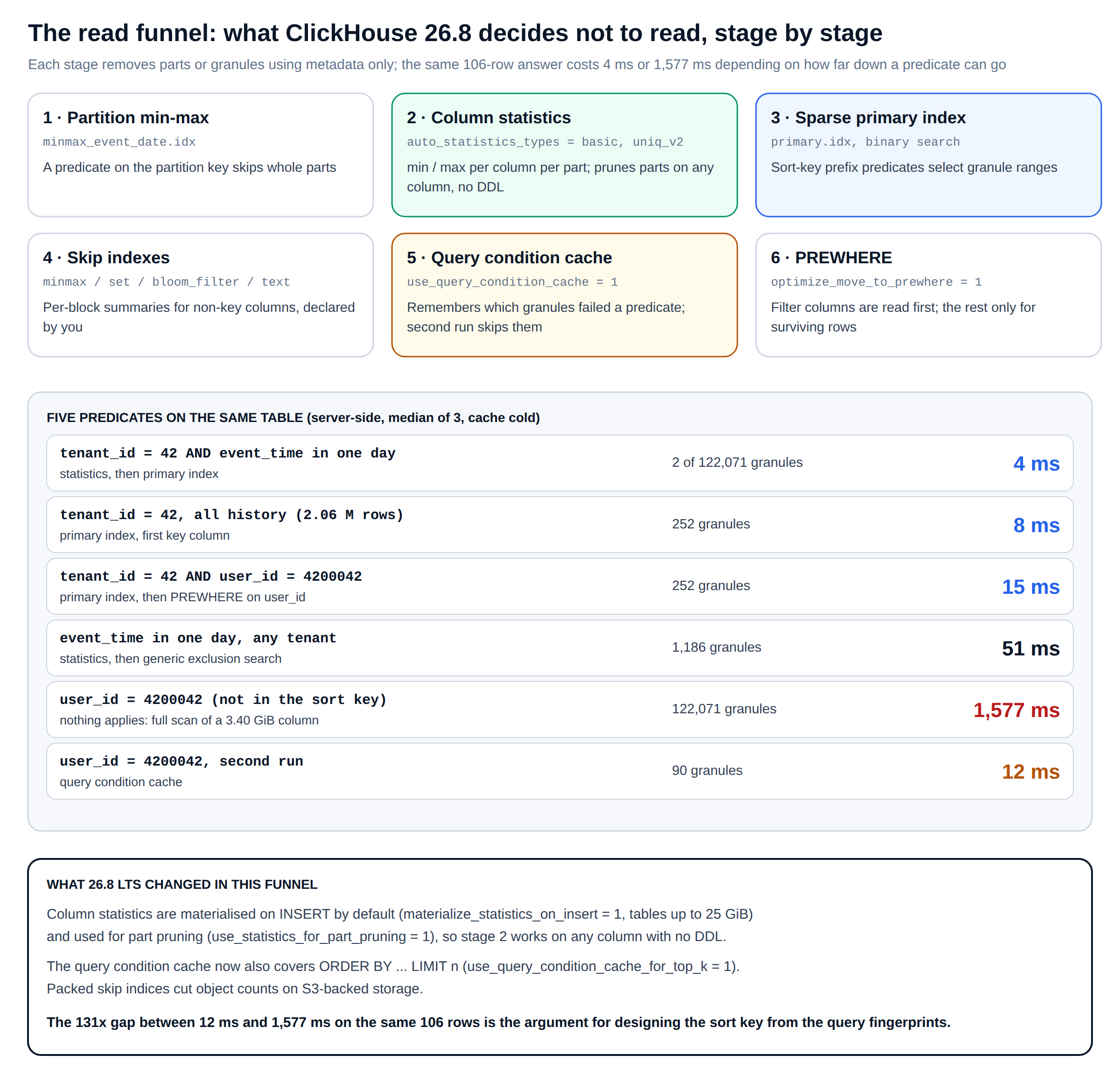
Two layers cooperate here. Part-level column statistics, which the 26.7 build maintains automatically, discard 35 of the 40 parts because their event_time range cannot contain 10 March; the primary key then binary-searches the 4,873 granules of the five survivors down to 7. Eight milliseconds against a billion rows, and the table was never in memory. If one measurement explains why ClickHouse is so fast for tenant-scoped analytics, it is this one.
| Predicate on the billion-row table | Index path | Granules read | Median |
|---|---|---|---|
| tenant_id = 42 AND event_time within one day | Statistics 40 → 5 parts, PrimaryKey binary search | 7 of 122,127 | 8 ms |
| tenant_id = 42 (all 2,000,697 rows of the tenant) | PrimaryKey binary search on the first key column | 291 of 122,127 | 31 ms |
| tenant_id = 42 AND user_id = 4200042 (106 rows) | PrimaryKey on tenant_id, PREWHERE on user_id inside it | 291 of 122,127 | 28 ms |
| event_time within one day, no tenant (15.8 M rows) | Statistics 40 → 5 parts; second key column, generic search | 1,929 of 122,127 | 96 ms |
| user_id = 4200042 alone (106 rows) | No usable index; PREWHERE scan of the 3.41 GiB column | 122,087 of 122,127 | 2,875 ms |
Table 3. Five predicates, one table, and the ClickHouse performance range they span. The same 106 rows cost 28 ms or 2,875 ms depending on whether the query also names the first sort-key column. Nothing else changed.
The last two rows are the most instructive thing on this page for anyone designing a schema. A predicate that follows the sort-key prefix is resolved by the index; a predicate that does not is a full scan of that column, however selective it is. This is the single largest lever in ClickHouse performance engineering, and it is set at CREATE TABLE time, which is why ClickHouse is so fast for teams that chose their ORDER BY carefully and merely adequate for teams that did not.
If the PrimaryKey line of EXPLAIN indexes = 1 shows the same granule count before and after, the query is not using your ORDER BY. Fix the key, add a projection with a different order, or accept the scan. No server setting compensates for it.
Design choice 3
Design choice 3: partition pruning, skip indexes and the query condition cache
Above the primary index sit coarser filters, each cheap, each visible in the same plan output that drives every ClickHouse performance review. The partition key’s min/max is kept per part, so a month predicate on this table touches 5 to 7 of the 40 parts before any granule-level work. Automatic column statistics, visible as the Statistics line in the plans above, do the same for columns that are not the partition key. Skip indexes extend the idea to columns outside the sort key altogether: a min/max pair, a set of values or a Bloom filter per block of granules, consulted to prove that a block cannot contain a match.
ClickHouse 25.3 introduced a further layer that surprised us during this lab, and it is on by default in every current release including 26.8 LTS. The query condition cache remembers, per predicate and per granule, which granules matched the last time the predicate ran. On the user_id scan from Table 3, the one with no index help at all, the second execution went from 2,020 ms to 19 ms with no change to the query, the table or the data.
sql · the query condition cache on the worst-case predicate
SELECT count(), sum(bytes_out) FROM lab.events WHERE user_id = 4200042
SETTINGS use_query_condition_cache = 1;
-- run 1: 2,020 ms   run 2: 19 ms   run 3: 23 ms

SELECT count(), sum(bytes_out) FROM lab.events WHERE user_id = 4200042
SETTINGS use_query_condition_cache = 0;
-- run 1: 1,946 ms   run 2: 1,975 ms

SELECT count() AS entries, formatReadableSize(sum(entry_size)) AS size
FROM system.query_condition_cache;
A 100x improvement on a repeated dashboard filter costs nothing and is on by default in this build, which is why every headline number in this article was measured with it switched off. It is also why a naive benchmark that runs each query three times and reports the best run will overstate ClickHouse performance on filtered queries by two orders of magnitude. Report the first run, or disable the cache, and say which; every ClickHouse performance figure in this article does.
| Skip index type | Summary stored per block | Pays when | Wasted when |
|---|---|---|---|
| minmax | min and max | The column correlates with the sort order (timestamps, monotonic IDs) | Values spread through every block |
| set(N) | up to N distinct values | A low-cardinality column clustered in runs | Per-block cardinality exceeds N |
| bloom_filter(p) | Bloom filter with false-positive rate p | Equality and IN on high-cardinality values read from slow or cold storage | Range predicates; warm narrow columns that PREWHERE already handles |
| text (current releases; the 26.x documentation marks tokenbf_v1 and ngrambf_v1 as deprecated) | Inverted token index | hasToken, LIKE and full-text on log lines | Very short strings; ingest-heavy tables without tuning |
Table 4. Skip-index types on ClickHouse 26.x and their ClickHouse performance profile. On our 20-million-row sibling table a Bloom filter pruned 92% of granules and moved wall-clock by nothing, because PREWHERE had already done the work on a warm column; on the billion-row table, where the user_id column is 3.41 GiB and cold, it is precisely the tool for the 2,875 ms row of Table 3.
Design choice 4
Design choice 4: per-column codecs, measured on 99.5 million rows
A column stream holds values of one type, often sorted or slowly varying, and ClickHouse lets each column declare its own codec chain: a shape-aware codec (Delta, DoubleDelta, Gorilla, T64, GCD, FPC) followed by a general-purpose one (LZ4 by default in open-source ClickHouse, ZSTD by default in ClickHouse Cloud). We copied the first 99.5 million rows of the events table into a second table with codecs chosen per column and compared, because compression is the least-discussed part of why ClickHouse is so fast and often the cheapest to improve.
sql · per-column codecs on the same 99,532,800 rows
CREATE TABLE lab.events_codec
(
    tenant_id    UInt16                 CODEC(Delta(2), ZSTD(1)),
    event_time   DateTime               CODEC(Delta(4), ZSTD(1)),
    event_date   Date MATERIALIZED toDate(event_time),
    user_id      UInt32                 CODEC(ZSTD(1)),
    event_type   LowCardinality(String) CODEC(ZSTD(1)),
    country      LowCardinality(String) CODEC(ZSTD(1)),
    device       LowCardinality(String) CODEC(ZSTD(1)),
    url_path     LowCardinality(String) CODEC(ZSTD(1)),
    http_status  UInt16                 CODEC(T64, ZSTD(1)),
    latency_ms   UInt16                 CODEC(T64, ZSTD(1)),
    bytes_out    UInt32                 CODEC(T64, ZSTD(1))
)
ENGINE = MergeTree
PARTITION BY toYYYYMM(event_date)
ORDER BY (tenant_id, event_time);

┌─table────────┬─compressed─┬─uncompressed─┬─ratio─┐
│ events (LZ4) │ ~1.58 GiB  │ 2.32 GiB     │  1.47 │   -- pro-rated from the full table
│ events_codec │ 887.10 MiB │ 2.32 GiB     │  2.68 │
└──────────────┴────────────┴──────────────┴───────┘| Column | LZ4 default (full table, ratio) | Tuned codec (99.5 M slice, ratio) | What changed |
|---|---|---|---|
| tenant_id | 8.61 MiB (221x) | 206 KiB (945x) | Delta on the first sort-key column turns a sorted UInt16 into zeros |
| event_date | 9.00 MiB (212x) | 909 KiB (214x) | Already near its floor |
| http_status | 234 MiB (8.2x) | 16.7 MiB (11.4x) | T64 packs a 16-bit column that holds four distinct values |
| event_time | 3.60 GiB (1.0x) | 90.6 MiB (4.2x) | Delta(4) on timestamps that are monotonic within each tenant; LZ4 alone saw noise |
| bytes_out | 2.75 GiB (1.4x) | 165 MiB (2.3x) | T64 drops the unused high bits of a UInt32 |
| user_id | 3.41 GiB (1.1x) | 252 MiB (1.5x) | Hash-random within a 20,000 range: little for any codec to find |
Table 5. Codec effect per column, the ClickHouse performance lever that costs nothing at query time. event_time is the lesson: a timestamp column that LZ4 could not compress at all shrank 4.2x once told it was a sequence of deltas.
The codec table was also faster to query, not slower, a ClickHouse performance result that runs against the usual intuition about ZSTD. The same avg(latency_ms), count() ran in 155 ms on the ZSTD table against 186 ms on the LZ4 slice, and the 17-way GROUP BY in 358 ms against 413 ms.
On the 20-million-row table in our sibling article, which fitted in page cache, LZ4 won by 20% because the scan was CPU-bound; here the table does not fit and the scan is bound by bytes moved, so the smaller table wins. Which regime a production node is in is a measurement, not an opinion, and system.parts_columns on your own data is where the answer lives.
Design choice 5
Design choice 5: vectorised execution, and what it costs to lose it
Once bytes are in memory ClickHouse never reconstructs rows, and this is where why ClickHouse is so fast stops being about I/O. Every processor consumes and produces a chunk of column arrays holding up to max_block_size rows, 65,409 by default, and runs one tight typed loop per chunk with SIMD kernels selected at runtime. The interpretive cost of deciding what to execute is paid once per chunk rather than once per row. The cheapest way to price that design, and to see how much of why ClickHouse is so fast lives in it, is to shrink the chunk on a billion rows.
| max_block_size | Rows per processor call | event_type, count(), avg(latency_ms) GROUP BY event_type over 1 B rows | Relative |
|---|---|---|---|
| 65409 (default) | 65,409 | 4,330 ms | 1.0x |
| 8192 | 8,192 | 5,680 ms | 1.3x |
| 1024 | 1,024 | 15,475 ms | 3.6x |
Table 6. Why ClickHouse is so fast per byte: same query, same data, same two threads, same bytes read. At 1,024 rows per call the per-call overhead is 11 extra seconds on a billion rows. At the default it is amortised to nothing, which is a large part of why ClickHouse is so fast per byte.
sql · EXPLAIN PIPELINE · the shape on two threads
EXPLAIN PIPELINE
SELECT event_type, count(), avg(latency_ms)
FROM lab.events
GROUP BY event_type
SETTINGS max_threads = 2;

(Expression)  ExpressionTransform × 2
(Aggregating) Resize 2 → 2
              AggregatingTransform × 2
(Expression)  ExpressionTransform × 2
(ReadFromMergeTree)
              MergeTreeSelect(pool: ReadPool, algorithm: Thread) × 2 0 → 1
PREWHERE is the vectorised engine’s I/O-side twin and a ClickHouse performance feature most teams inherit without knowing it. When a query filters on cheap columns and selects expensive ones, the optimiser reads the filter columns first, evaluates the predicate, and fetches the remaining columns only for granules that survived. We asked for every column of every row that was a purchase, returned HTTP 500 and took more than 1.4 seconds: 2,924 rows out of a billion.
sql · optimize_move_to_prewhere on and off, SELECT * over 1 B rows
SELECT * FROM lab.events
WHERE http_status = 500 AND event_type = 'purchase' AND latency_ms > 1400
SETTINGS max_threads = 2, optimize_move_to_prewhere = 1;   -- median 9,613 ms

SELECT * FROM lab.events
WHERE http_status = 500 AND event_type = 'purchase' AND latency_ms > 1400
SETTINGS max_threads = 2, optimize_move_to_prewhere = 0;   -- median 15,813 ms
Six seconds of ClickHouse performance from a default setting most teams have never heard of, on a query that reads 233 MiB of http_status to avoid reading 15 GiB of everything else. On a node with more cores and faster storage the absolute times shrink; the ratio does not.
Design choice 6
Design choice 6: parallelism over mark ranges, from two cores to three clouds
ClickHouse parallelises at three multiplicative levels, and the unit of work at every level is the same object: a range of marks inside a part. A thread, a shard and a replica each take mark ranges; none of them introduces a new kind of coordination, which is why ClickHouse is so fast to scale out as well as up. On our two cores the first level is the only one we can show, and it is close to ideal; it is also why ClickHouse is so fast on a cluster for the same reason it is fast on one node.
| max_threads | GROUP BY event_type with avg over 1 B rows | Scaling |
|---|---|---|
| 1 | 8,640 ms | 1.00x |
| 2 | 4,457 ms | 1.94x |
Table 7. ClickHouse performance scaling across threads on identical mark ranges. Each thread runs a private pipeline and a private aggregation hash table; the two are merged once at the end.
Level 1: threads within a node
A SELECT spreads its mark ranges over max_threads (auto = physical cores). Each thread owns its hash table; the merge is bucket-parallel once the table converts to two-level. Measured: 1.94x on two cores, which is what a 64-core node also delivers per core until storage saturates.
Level 2: shards
A Distributed table fans the query to every shard, which executes it locally and returns partial aggregate states rather than rows. distributed_aggregation_memory_efficient streams the merge so the initiator stays bounded.
Level 3: parallel replicas
Replicas of one shard cooperate on a single query, the initiator handing out mark ranges dynamically. It turns a standby into compute. Opt-in in open-source ClickHouse (enable_parallel_replicas = 0 is the 26.7 default we read from system.settings) and the machinery behind LogHouse’s 33 geoshards.
The ClickHouse performance blast radius of turning any level up is memory: one aggregation hash table per thread, per replica. Raise max_threads or enable parallel replicas together with max_memory_usage and max_concurrent_queries, stage on one replica, and read system.query_log.memory_usage at p99 before rolling out.
Design choice 7
Design choice 7: merge-time precomputation, 5,567 ms to 7 ms
MergeTree is LSM-shaped. Inserts create immutable sorted parts; background merges combine them, re-sort them, rebuild marks and indexes, apply TTL and recompress. That gives the engine a place to do work between ingest and query that a row store does not have, and incremental materialized views use it: every inserted block is run through the view’s SELECT and the resulting aggregate states are written to a target table whose merges fold states with the same key together.
sql · a daily per-tenant view over the billion-row table
CREATE TABLE lab.events_daily
(
    tenant_id UInt16,
    day       Date,
    events    AggregateFunction(count),
    errors    AggregateFunction(countIf, UInt8),
    users     AggregateFunction(uniqCombined(12), UInt32),
    bytes_out AggregateFunction(sum, UInt64)
)
ENGINE = AggregatingMergeTree
PARTITION BY toYYYYMM(day)
ORDER BY (tenant_id, day);

CREATE MATERIALIZED VIEW lab.mv_events_daily TO lab.events_daily AS
SELECT tenant_id, event_date AS day,
       countState()                       AS events,
       countIfState(http_status >= 500)   AS errors,
       uniqCombinedState(12)(user_id)     AS users,
       sumState(toUInt64(bytes_out))      AS bytes_out
FROM lab.events
GROUP BY tenant_id, day;

-- one-time backfill of the existing billion rows, month by month: 26.5 s
-- target: 90,500 rows, 227.36 MiB (the source table is 15.84 GiB)

-- events, users and errors per tenant for one quarter
--   base table: 502,336,000 rows, 61,324 granules      median 4,455 ms
--   view:            45,500 rows,      9 granules      median   271 ms
-- all-time daily totals
--   base table: 1,000,000,000 rows                     median 5,567 ms
--   view:              90,500 rows                     median     7 ms
-- results compared row for row: identical
The view is 1.4% of the table on disk and answers the two dashboard questions 16x and 795x faster respectively, including a distinct-user count that would otherwise hash half a billion values. Two disciplines keep this ClickHouse performance pattern honest in production. The reading query’s GROUP BY must match the target’s ORDER BY, and a view sees only new inserts, so existing data needs the one-time backfill shown and any later correction of source rows needs a matching correction in the target.
Granularity is the design decision, and the difference between a view that explains why ClickHouse is so fast on a dashboard and one that merely costs disk. Our first attempt was an hourly view keyed by tenant, hour and event type. It grew to 21.7 million rows and 2.12 GiB, carried a quantile state per row, and answered the quarterly question in 4,078 ms against 4,455 ms from the base table, a saving not worth its storage.
Collapsing to tenant and day, and dropping the quantile in favour of the count, error and distinct-user states the dashboard actually displays, produced the 271 ms result. A materialized view is a query plan frozen at insert time; it has to be the plan the dashboard needs, and when it is, it is why ClickHouse is so fast on dashboards that summarise billions of rows.
The merge is also where ingest design meets ClickHouse performance, and where why ClickHouse is so fast to read becomes a question of how it is written. One thousand single-row inserts took 2.3 s and produced one thousand parts, which background merges reduced to six, the ClickHouse performance failure mode that fills support queues; one insert of 10,000,000 rows took 0.17 s, a rate of 57 million rows per second into a sorted part.
LogHouse’s 190 million rows per second across 5,800 inserts per second is the same arithmetic at fleet size: about 33,000 rows per insert. Batch at the client or set async_insert = 1 so the server batches for you; parts_to_throw_insert (3,000 by default) is the guard rail that eventually rejects the alternative.
Limits
Where ClickHouse is not fast, on the same billion rows
Understanding why ClickHouse is so fast tells you exactly where it is not, and our lab produced three examples without looking for them. A point filter on a column outside the sort key is a full column scan: 2,875 ms for 106 rows in Table 3, against 28 ms when the query also names the tenant.
The second example is a ClickHouse performance edge inside the aggregation engine. A GROUP BY on two LowCardinality columns at once, country and device, took 25 seconds where the single-key GROUP BY took 3, because the aggregation falls off the fixed-width fast path onto a serialised composite key; the fix is a precomputed view or a single derived key, and it is the kind of thing a profile finds in a minute and a benchmark table never shows.
The third example is aggregation cost rather than I/O. A 95th-percentile latency across 160 country-device groups took 27 seconds because a billion values were sampled into 160 quantile states; that query belongs in a materialized view, not on a dashboard.
The structural limits of ClickHouse performance are the ones we measured on the 20-million-row sibling table in the row-store comparison: a point lookup by primary key at 5 to 9 ms against 0.1 ms in PostgreSQL, and a single-row UPDATE as an 8-second mutation against 0.65 ms. Hash joins build the right-hand table in memory per query, so a billion-row fact-to-fact join without dictionaries, denormalisation or grace_hash exhausts max_memory_usage. If a workload is mostly point reads and row-level writes, no ClickHouse performance tuning rescues it; it belongs on a row store with CDC into ClickHouse for the analytical half, and MinervaDB’s PostgreSQL and MySQL practices exist for exactly that split.
Measure it yourself
Measuring why ClickHouse is so fast, or is not, on your own cluster
Every claim on this page maps to a column in system.query_log. This is the first query we run in a ChistaDATA ClickHouse performance engagement, per query shape: how many bytes Phase 1 let through and how much CPU Phase 2 spent on them.
sql · the first query of every performance engagement
SELECT
    normalizedQueryHash(query)                                   AS query_hash,
    count()                                                      AS executions,
    quantile(0.95)(query_duration_ms)                            AS p95_ms,
    formatReadableSize(avg(read_bytes))                          AS avg_read,
    avg(read_rows)                                               AS avg_read_rows,
    avg(ProfileEvents['SelectedMarks'])                          AS avg_marks,
    avg(ProfileEvents['SelectedParts'])                          AS avg_parts,
    avg(ProfileEvents['OSCPUVirtualTimeMicroseconds']) / 1000    AS avg_cpu_ms,
    formatReadableSize(max(memory_usage))                        AS max_memory,
    any(query)                                                   AS sample_query
FROM system.query_log
WHERE type = 'QueryFinish'
  AND event_time >= now() - INTERVAL 24 HOUR
  AND query_kind = 'Select'
GROUP BY query_hash
ORDER BY p95_ms DESC
LIMIT 25;| Signal | Points at | Design choice to revisit |
|---|---|---|
| avg_marks close to the table’s total marks | Primary index not used | 2: reorder ORDER BY, or 7: a projection |
| High read_bytes with few read_rows | Wide columns, SELECT *, or a poor codec | 1 and 4 |
| Second run much faster than the first | Query condition cache, page cache or query cache | 3: report first-run numbers |
| avg_cpu_ms far above p95_ms | Good parallelism, CPU-bound | 7: precompute, or 5: block size and JIT |
| p95_ms far above avg_cpu_ms | I/O wait, merge pressure or lock wait | Storage tier, system.merges, choice 3 on cold data |
| max_memory near max_memory_usage | Hash table or join spill risk | 6: thread and replica settings, join_algorithm |
Table 8. Reading query-log output back to the seven design choices behind why ClickHouse is so fast.
| Setting | Default read from system.settings on 26.7 | Effect on speed |
|---|---|---|
| max_threads | auto (physical cores) | Level-1 parallelism; 1.94x on two cores here |
| max_block_size | 65409 | Rows per chunk; Table 6 shows the cost of shrinking it |
| optimize_move_to_prewhere | 1 | Filter on cheap columns before reading expensive ones; 6 s on a billion rows here |
| use_query_condition_cache | 1 | Granule-level memo of predicate results; 100x on repeated filters |
| use_skip_indexes | 1 | Consult skip indexes; set 0 to measure their real contribution |
| compile_expressions | 1 | LLVM JIT for expression chains |
| optimize_read_in_order | 1 | Stream sorted parts through ORDER BY without a sort |
| join_algorithm | direct, parallel_hash, hash | Join strategy order |
| enable_parallel_replicas | 0 | Level-3 parallelism, opt-in in open source |
| use_query_cache | 0 | Whole-result caching, opt-in; never for queries containing now() |
Table 9. ClickHouse performance settings and the defaults we read from system.settings on the 26.7 build. Session settings apply on the next query; server configuration needs a restart.
Reproduce
Reproduce the billion rows
The generator below produces the identical table on any ClickHouse 26.x, including chDB, so every claim here about why ClickHouse is so fast can be checked rather than believed. On two vCPU it ran at 2.01 million rows per second and finished in 498.6 s; OPTIMIZE FINAL took a further 156 s. Budget 16 GiB of disk plus one partition of headroom for the merge. Test on a copy of your own data before drawing conclusions for production, and keep a tested restore path before touching any schema that serves traffic.
sql · deterministic generator for 1,000,000,000 rows (run in 20 chunks of 50 M)
INSERT INTO lab.events
SELECT
    toUInt16(1 + intHash32(number) % 500)                                   AS tenant_id,
    toDateTime('2026-01-01 00:00:00') + toIntervalSecond(intDiv(number, 64)) AS event_time,
    toUInt32(tenant_id * 100000 + intHash64(number) % 20000)                AS user_id,
    ['page_view','page_view','page_view','page_view','page_view','page_view','click','click',
     'api_call','api_call','search','login','purchase','error','logout','signup','export']
        [1 + intHash32(number * 7) % 17]                                     AS event_type,
    ['US','US','US','IN','IN','DE','GB','BR','FR','JP','CA','AU','SG','NL','ES','IT','MX','KR','ID','AE',
     'SE','PL','TR','ZA','AR','CH','BE','TH','MY','PH','VN','NG','EG','SA','IL','IE','AT','DK','NO','FI']
        [1 + intHash32(number * 11) % 40]                                    AS country,
    ['ios','android','web','web','web','desktop'][1 + intHash32(number * 13) % 6] AS device,
    concat('/api/v1/', ['orders','users','catalog','cart','search','checkout','profile','reports','events','billing']
        [1 + intHash32(number * 17) % 10], '/', toString(intHash32(number * 19) % 30)) AS url_path,
    multiIf(intHash32(number * 23) % 1000 < 950, 200,
            intHash32(number * 23) % 1000 < 985, 404,
            intHash32(number * 23) % 1000 < 995, 500, 302)                   AS http_status,
    toUInt16(8 + intHash32(number * 29) % 240 + if(intHash32(number * 31) % 40 = 0, 1200, 0))     AS latency_ms,
    toUInt32(180 + intHash32(number * 37) % 4000 + if(intHash32(number * 41) % 25 = 0, 60000, 0)) AS bytes_out
FROM numbers_mt(0, 50000000)          -- then 50000000, 100000000, ... up to 950000000
SETTINGS max_insert_threads = 2, max_threads = 2;

OPTIMIZE TABLE lab.events FINAL;

-- the toggles that isolate each design choice
SELECT ... SETTINGS use_query_condition_cache = 0;   -- always, for first-run numbers
SELECT ... SETTINGS use_skip_indexes = 0;            -- choice 3
SELECT ... SETTINGS max_block_size = 1024;           -- choice 5
SELECT ... SETTINGS optimize_move_to_prewhere = 0;   -- choice 5
SELECT ... SETTINGS max_threads = 1;                 -- choice 6
Further reading
Further reading
- Columnar databases vs row-based databases, measured on 20 million rows: the same mechanisms beside PostgreSQL 16, with the row-store side of every comparison above.
- How Cloudflare uses ClickHouse at quadrillion-row scale and A quadrillion rows across three clouds: scaling LogHouse, the published deployments quoted in Table 1.
- ClickBench, the independent benchmark whose methodology (cold run, then two hot runs, each reported) is the one to copy.
- ClickHouse documentation: a practical introduction to primary indexes, the mark-selection algorithm behind Figure 2.
- ClickHouse documentation: incremental materialized views, including the -State and -Merge combinator contract used in design choice 7.
- ChistaDATA University: instructor-led ClickHouse training, including MergeTree internals and ClickHouse performance engineering modules.
ChistaDATA Inc. is not affiliated with ClickHouse, Inc. ClickHouse® is a registered trademark of ClickHouse, Inc. Third-party scale figures are quoted from the linked publications. Lab behaviour was verified on open-source ClickHouse 26.7; test every change in staging before applying it to production and maintain a tested disaster-recovery posture.
Next step
Knowing why ClickHouse is so fast is the start; keeping it fast at a quadrillion rows is engineering
ChistaDATA runs 24×7×365 consultative support, ClickHouse performance engineering, platform engineering and managed services on 100% open-source ClickHouse, with a 15-minute S1 response and no vendor lock-in. If your p95 is not where this page says it should be, we find out which of the seven choices your tables are missing, with the same system tables shown here: ClickHouse consulting, ClickHouse support, ClickHouse managed services and ClickHouse migration.
Running ClickHouse in production? ChistaDATA provides ClickHouse consulting for architecture, performance and migrations, and 24×7 ClickHouse support with a 15-minute S1 response. For day-to-day operations see ClickHouse DBA services and ClickHouse managed services.
