ChistaDATA · ClickHouse query execution, stage by stage · September 2026
ClickHouse query execution has no magic in it. A statement is parsed and planned, parts are scanned in parallel, partial results are merged, and the answer goes back. Every ClickHouse query execution problem our support engineers are handed is one of those steps doing more work than it needs to, and the fix starts with knowing which step it is.
This article follows one table from its first INSERT through a GROUP BY, a JOIN and a query across shards, and explains what the server does at each stage and what that means for time and memory. The examples use a telemetry schema we see in some form at most customers. Settings and system tables are named exactly; defaults change between releases, so check the ones that matter on the version you run before you rely on them.
Why the model matters
ClickHouse query execution is simple enough to hold in your head
ClickHouse is a columnar SQL engine with a shared-nothing architecture, parallel and vectorised execution, and an execution model that does not hide much from the person writing the query. That last point is the useful one. Most ClickHouse query execution tickets we close do not need a new setting; they need the engineer to know which of the four stages is burning the time, and the model is small enough that any developer can learn it in an afternoon.
Three properties decide how ClickHouse query execution behaves. Columnar storage means a query pays only for the columns it names. Shared-nothing means a query against a cluster is really a set of local queries plus a merge. Parallel execution means memory scales with the number of threads as well as with the data, and it scales differently for an INSERT than for a GROUP BY.
What follows is ClickHouse query execution in four stages: the INSERT that creates the data, the GROUP BY that reads it, the JOIN that widens it, and the Distributed table that spreads it across a cluster. Each stage ends with the settings and system tables that expose it, and with what we would check first on a production cluster.
Stage 1
ClickHouse query execution starts before any SELECT: the INSERT
The working table is a device-telemetry event log. It is small enough to reason about and carries everything that matters: columns, an engine, a partition rule and a sort key. The engine line and the two clauses after it are the whole storage design, and they shape every later stage of ClickHouse query execution.
CREATE TABLE telemetry.events
(
    tenant_id    UInt32,
    device_id    UInt64,
    event_time   DateTime,
    event_type   LowCardinality(String),
    http_status  UInt16,
    latency_ms   UInt32
)
ENGINE = MergeTree()
PARTITION BY toYYYYMM(event_time)          -- how rows are broken into parts
ORDER BY (tenant_id, event_time);           -- how each part is sorted and indexed

INSERT INTO telemetry.events FORMAT JSONEachRow
{"tenant_id":1001,"device_id":77,"event_time":"2026-09-01 06:12:00","event_type":"api_call","http_status":200,"latency_ms":41}
{"tenant_id":1001,"device_id":78,"event_time":"2026-09-01 06:12:03","event_type":"page_view","http_status":200,"latency_ms":118}
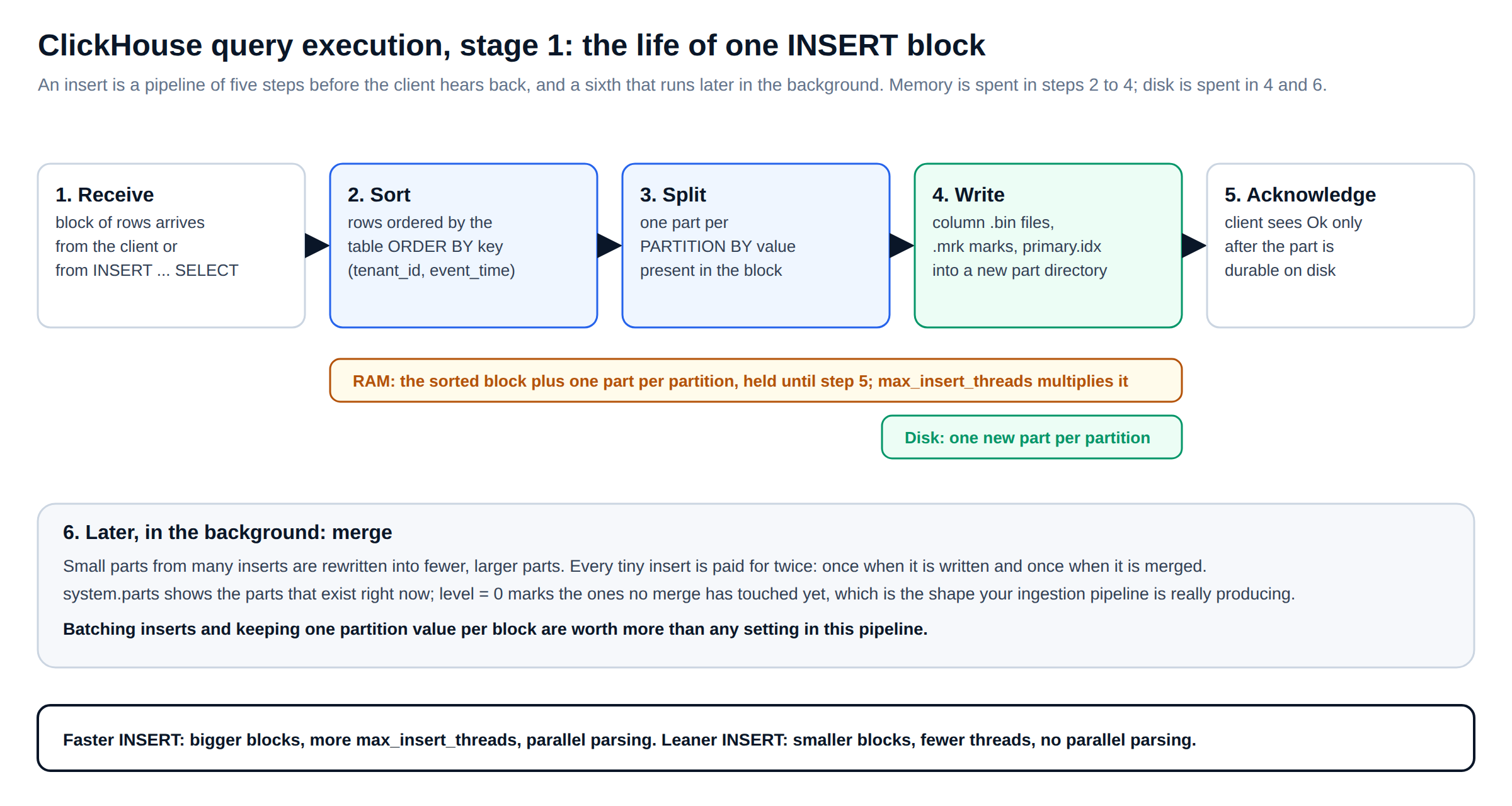
ClickHouse query execution for an INSERT is three steps: the server parses and plans the statement, loads the block, and responds. The load step is where the work of ClickHouse query execution is: rows are sorted by the table ORDER BY, split by partition key, written as a part in RAM, and then flushed as a part on storage. The client gets its acknowledgement only after the part is on disk. Nobody inserts two rows at a time in production; the same path runs for a ten-million-row batch.
Parallelising the load with max_insert_threads
An INSERT … SELECT can build several parts at once. Backfilling a month of history from a staging table is the usual case:
SET max_insert_threads = 4;

INSERT INTO telemetry.events
SELECT *
FROM staging.events_raw
WHERE event_time >= '2026-08-01'
  AND event_time <  '2026-09-01';
Two things happen as that setting goes up. Elapsed time falls until the source scan or the disk becomes the limit, after which more threads buy nothing. Memory rises with every step, because each thread holds its own part in RAM until the flush. Parallelism in ClickHouse query execution buys time with memory, and the curve flattens well before the thread count does. Do not set it from a rule of thumb; run the backfill at 1, 2, 4 and 8 on a staging copy and read the results from the query log.
That log is the first thing we open in any ClickHouse query execution review, and every claim in this article can be checked against it:
-- Per-fingerprint cost over the last hour: what ran, how often, and what it cost
SELECT
    normalizedQueryHash(query)                       AS fingerprint,
    count()                                          AS runs,
    round(avg(query_duration_ms))                    AS avg_ms,
    round(quantile(0.95)(query_duration_ms))         AS p95_ms,
    formatReadableSize(max(memory_usage))            AS peak_memory,
    formatReadableQuantity(sum(read_rows))           AS rows_read,
    any(query)                                       AS example
FROM system.query_log
WHERE type = 'QueryFinish'
  AND event_time >= now() - INTERVAL 1 HOUR
  AND user = '${CH_USER}'
GROUP BY fingerprint
ORDER BY sum(query_duration_ms) DESC
LIMIT 20;
system.query_log keeps duration, rows and bytes read, result size and peak memory for every finished query, so the question "which query is the problem" is a GROUP BY away. When someone tells us a query "used a lot of memory", this is where we go before we believe it.
What the INSERT left behind
Parts, granules, marks and compressed blocks
A table is a set of parts, and parts are what ClickHouse query execution reads. Every row in a part belongs to the same partition value, one calendar month in the schema above. Inside a part the columns are stored sorted by the ORDER BY expression, and a sparse primary index lets ClickHouse query execution find rows by the leading columns of that expression without reading everything.
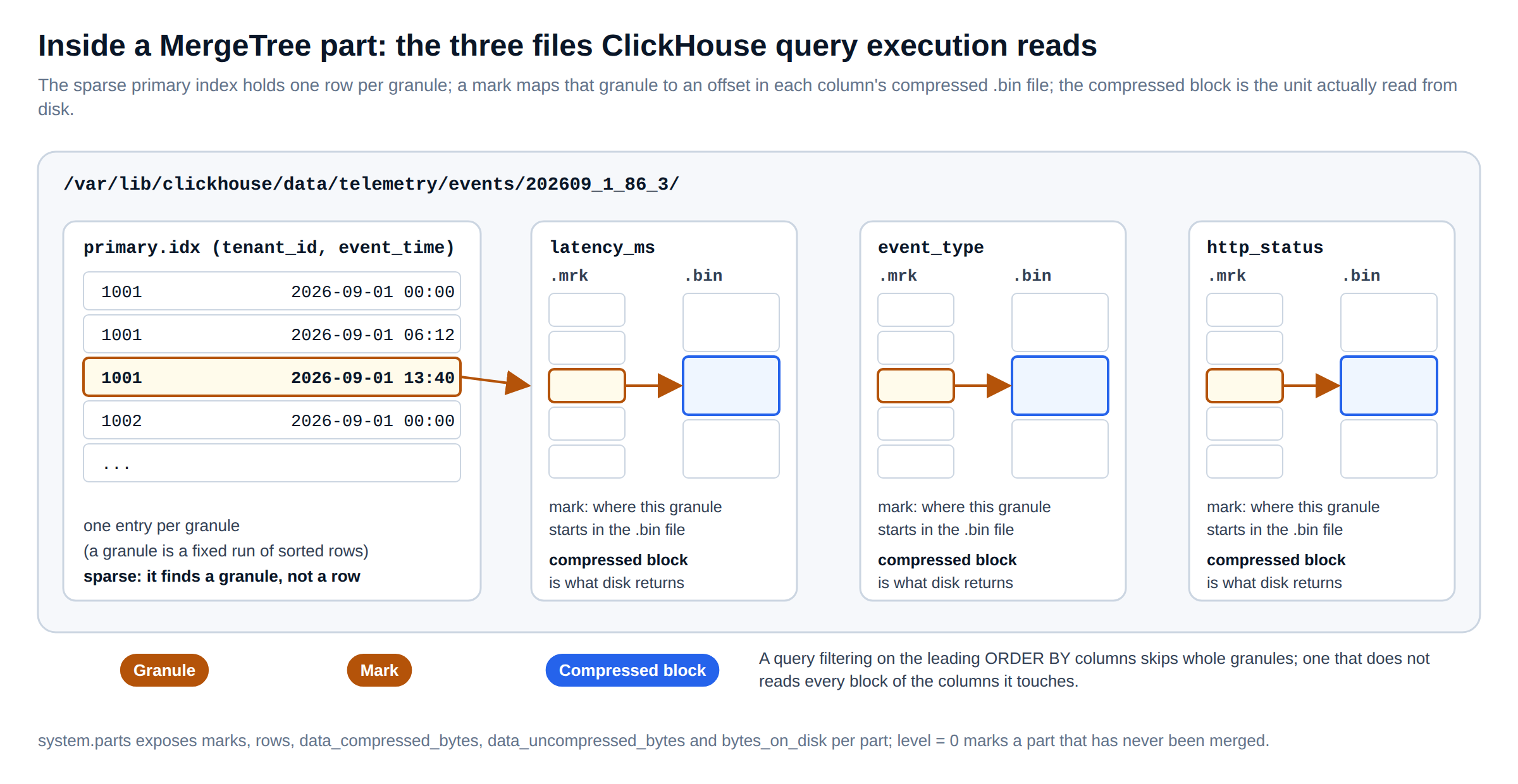
Three words are worth fixing in place, because ClickHouse query execution is described in them. A granule is the run of sorted rows that one primary-index entry stands for. A mark is the pointer from that granule into each column's .bin file. A compressed block is the unit that is read and decompressed. A query filtering on tenant_id in a table ordered by (tenant_id, event_time) reads the granules the index points at and nothing else; a query filtering on device_id, which is not in the sort key, reads every block of the columns it touches.
Why it is called MergeTree
Because it merges. Two parts become one rewritten, bigger part in the background, and updates and deletes rewrite parts too. Bigger parts are more efficient for ClickHouse query execution to read, so the design goal is to arrive at them cheaply.
In practice that means three things. Choose a PARTITION BY that produces large partitions and keeps the total part count per table in the hundreds, not the thousands; partitioning by month is the safe default when nothing about the workload argues otherwise. Insert large blocks so there is less to merge afterwards; a single INSERT carrying millions of rows is normal, not exotic. Keep one partition key per block, because a block that spans months becomes one part per month. Read the logs and the actual part sizes before touching max_insert_block_size; its default is usually adequate.
The query that shows the shape of a table's parts is short, and one column in it does most of the work:
-- Part shape per partition: how many parts, how big, and how many are still unmerged
SELECT
    partition,
    count()                                                    AS parts,
    countIf(level = 0)                                         AS unmerged_parts,
    formatReadableQuantity(sum(rows))                          AS rows,
    formatReadableSize(sum(bytes_on_disk))                     AS on_disk,
    round(sum(data_uncompressed_bytes) / sum(bytes_on_disk), 2) AS compression_ratio,
    formatReadableSize(min(bytes_on_disk))                     AS smallest_part
FROM system.parts
WHERE active
  AND database = 'telemetry'
  AND table = 'events'
GROUP BY partition
ORDER BY partition DESC;
level = 0 marks a part no merge has touched yet, so unmerged_parts and smallest_part together show what the ingestion pipeline is really producing: sensible blocks, or a spray of tiny parts that merges then have to pay for.
To make INSERT faster: raise max_insert_threads for parallel part creation, enable input_format_parallel_parsing for TSV, CSV and Values input, and write bigger blocks. To make INSERT use less memory: lower max_insert_threads so fewer parts sit in RAM at once, disable parallel parsing, and write smaller blocks. The two lists are mirror images, which is the honest way to say there is no free setting here.
Stage 2
ClickHouse query execution for GROUP BY: scan in parallel, merge once
Aggregation is the defining operation of analytic SQL and the centre of ClickHouse query execution: an aggregate function applied to a measurement, grouped by one or more dimensions. The smallest useful example on the telemetry table is average latency per event type.
SELECT
    event_type,
    avg(latency_ms) AS avg_latency
FROM telemetry.events
GROUP BY event_type
ORDER BY avg_latency DESC;
ClickHouse query execution for this statement parses and plans, then scans the parts in parallel. Each scan thread reads its share of the granules and keeps an in-RAM hash table keyed by the GROUP BY value. The value stored is not the answer but a partial aggregate state. For avg() that is a running sum and a count. The merge step adds the partial states from every thread, finalises the function, sorts, and returns.
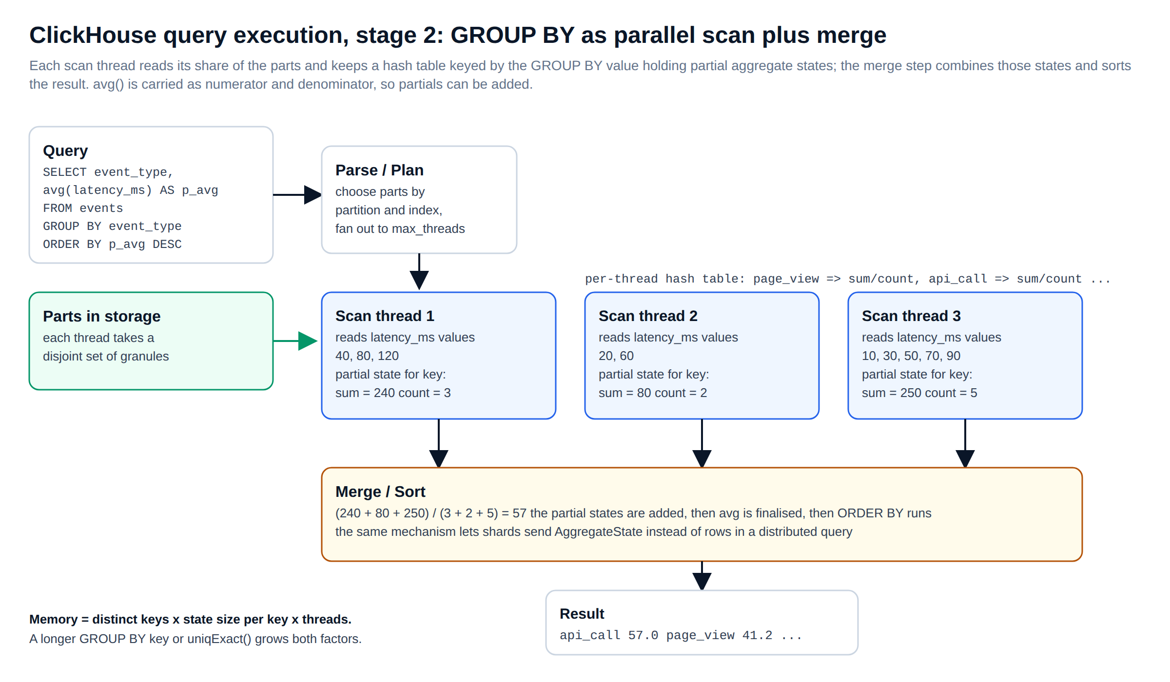
The arithmetic deserves spelling out because it is the whole reason the design works. Suppose three threads see the latencies (40, 80, 120), (20, 60) and (10, 30, 50, 70, 90) for one event type. Each produces a partial: 240/3, 80/2 and 250/5. The merge computes (240 + 80 + 250) / (3 + 2 + 5) = 57. No thread needed to see another thread's rows, and no thread needed to know how many threads there were. Every aggregate function in ClickHouse has a state that can be combined this way, which is also what -State and -Merge combinators and AggregatingMergeTree are built on.
What decides speed and memory in aggregation
Once you see the hash table per thread, the performance drivers of ClickHouse query execution are obvious. Memory is roughly the number of distinct keys, times the size of the state per key, times the number of threads holding a table. Grouping by event_type alone gives a handful of keys and a state of two integers. Add device_id and toStartOfHour(event_time) to the key and swap in uniqExact(tenant_id), and both factors grow: millions of keys, each carrying a hash set. The same table, the same rows read, and a query that can go from kilobytes to gigabytes of RAM.
-- Few keys, two-integer state per key
SELECT event_type, avg(latency_ms) AS avg_latency
FROM telemetry.events
GROUP BY event_type
ORDER BY avg_latency DESC
LIMIT 50;

-- Many keys, a hash set per key: same rows read, far more memory
SELECT device_id, toStartOfHour(event_time) AS h,
       avg(latency_ms)      AS avg_latency,
       uniqExact(tenant_id) AS tenants
FROM telemetry.events
GROUP BY device_id, h
ORDER BY avg_latency DESC
LIMIT 50;
Threads matter too, and memory does not always move the way you expect. Raising max_threads shortens the scan roughly until the cores or the disk are saturated; per-query memory may rise a little because there are more hash tables, or fall a little because each one is smaller and merges sooner. It is the opposite shape from the INSERT case, where every thread adds a whole part. Do not carry a rule of thumb from one stage of ClickHouse query execution to another; measure each on your own workload with system.query_log open.
The three memory limits
Three settings bound ClickHouse query execution, and Memory limit exceeded is the most common error string in our ticket queue, so they are worth naming. max_memory_usage caps a single query. max_memory_usage_for_user caps all queries for one user. max_server_memory_usage caps the whole server process. Which one fired is written in the error message; read it before changing anything, because the fix for each is different.
The list for making aggregation faster in ClickHouse query execution is short: remove or exchange heavy aggregate functions (uniq instead of uniqExact when an estimate is acceptable), reduce the number of distinct values in the GROUP BY, raise max_threads, and reduce I/O by filtering rows earlier and improving compression. The list for reducing memory is the same list with one addition, spilling partial aggregates to disk:
-- Let a large GROUP BY overflow to disk instead of failing
SET max_bytes_before_external_group_by = 10000000000;   -- bytes; any value > 0 enables the spill
We treat the spill as a safety net, not a fix. If a dashboard query needs it every run, the key or the function is wrong for the shape of the data, and the right move is usually a materialized view that carries the partial aggregate states already merged.
Stage 3
How ClickHouse query execution handles a JOIN, and why the order matters
A JOIN combines rows from a left table and a right table on a condition, and ClickHouse query execution treats the two sides very differently. The telemetry example attaches a device model to a per-device event count:
SELECT
    e.device_id,
    any(d.model)   AS model,
    count()        AS events
FROM telemetry.events e
JOIN telemetry.devices d ON d.device_id = e.device_id
GROUP BY e.device_id
ORDER BY events DESC
LIMIT 10;
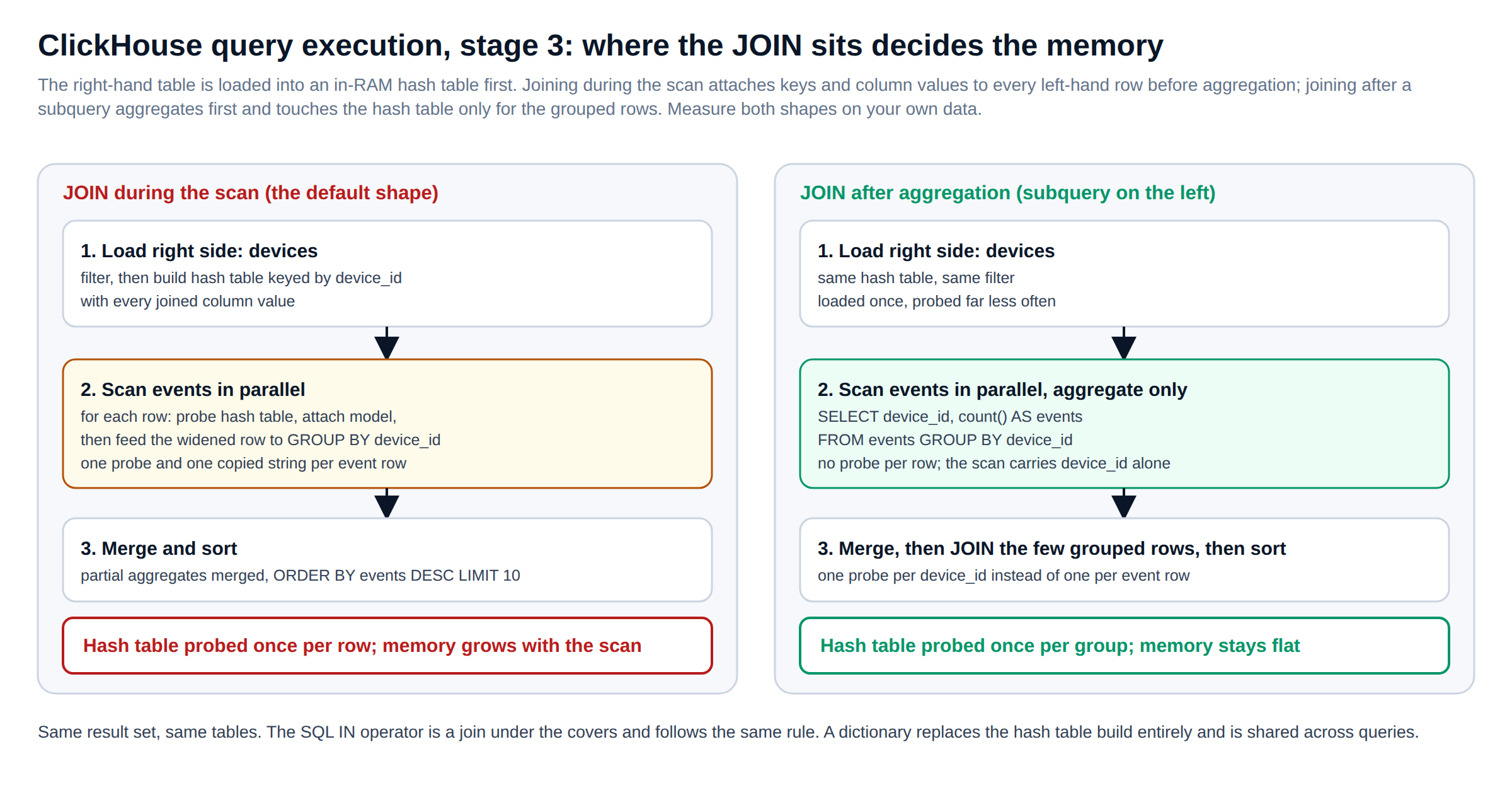
In ClickHouse query execution the engine loads the right-side table first, filters it, and builds an in-RAM hash table keyed by the join column, carrying the keys and every column value the query needs from that side. Then it scans the left-side table in parallel, probing the hash table for each row, attaching the joined columns, and feeding the widened row into aggregation. Finally it merges and sorts. The right side is expected to be small; the left side is expected to be big.
Look at what the scan is doing: for every one of the millions of events a device produced, it attaches the model string before the GROUP BY collapses those events into one row. That is work done per event for a value that is only needed per device, and it is why the probe-per-row shape uses memory in proportion to the scan.
Join after aggregating, with a subquery
The fix is to aggregate first and join the few surviving rows, so that ClickHouse query execution probes the hash table once per group instead of once per row. ClickHouse lets you say exactly that with a subquery on the left side:
-- Join during the scan: one probe per event row
SELECT e.device_id, any(d.model) AS model, count() AS events
FROM telemetry.events e
JOIN telemetry.devices d ON d.device_id = e.device_id
GROUP BY e.device_id
ORDER BY events DESC
LIMIT 10;

-- Join after aggregation: one probe per device
SELECT e.device_id, d.model, e.events
FROM
(
    SELECT device_id, count() AS events
    FROM telemetry.events
    GROUP BY device_id
) AS e
JOIN telemetry.devices d ON d.device_id = e.device_id
ORDER BY events DESC
LIMIT 10;
Same answer, and on every workload we have measured it on, the second shape is materially faster and uses a fraction of the memory; how much depends on the ratio of rows to groups, so run both on your data before deciding. The difference is not an optimiser trick. The scan carries device_id alone instead of device_id plus a model string, and the hash table is probed thousands of times instead of millions. This is the single rewrite we apply most often in ClickHouse query execution reviews, and it is the one a query author can see for themselves once they know how the scan works.
The rest of the list for JOINs in ClickHouse query execution follows from the same picture. Keep the right-side tables small overall. Minimise the columns pulled from the right side, because each one lives in the hash table. Add filter conditions to the right side so fewer rows are loaded. And where the right side is a lookup that many queries share, use a dictionary instead of a JOIN: a dictionary is loaded once and reused across queries, so the hash-table build disappears from every query that uses it.
The same rules reach further than the JOIN keyword. WHERE device_id IN (SELECT …) builds a set from the subquery and probes it per row, so the right side of an IN is a small table held in RAM exactly like the right side of a join, and it deserves the same filtering.
Stage 4
Distributed ClickHouse query execution: local queries plus a merge
A production cluster has three kinds of table on every node. events is a Distributed table holding no data. events_local is a sharded, replicated table holding part of the data. devices is fully replicated, so every node has all of it. That layout, a big fact table sharded and small dimension tables replicated everywhere, is the one we recommend by default because of what the next paragraphs describe.
CREATE TABLE telemetry.events_local ON CLUSTER '{cluster}'
(
    tenant_id UInt32, device_id UInt64, event_time DateTime,
    event_type LowCardinality(String), http_status UInt16, latency_ms UInt32
)
ENGINE = ReplicatedMergeTree('/clickhouse/tables/{shard}/telemetry/events_local', '{replica}')
PARTITION BY toYYYYMM(event_time)
ORDER BY (tenant_id, event_time);

CREATE TABLE telemetry.events ON CLUSTER '{cluster}'
AS telemetry.events_local
ENGINE = Distributed('{cluster}', 'telemetry', 'events_local', cityHash64(tenant_id));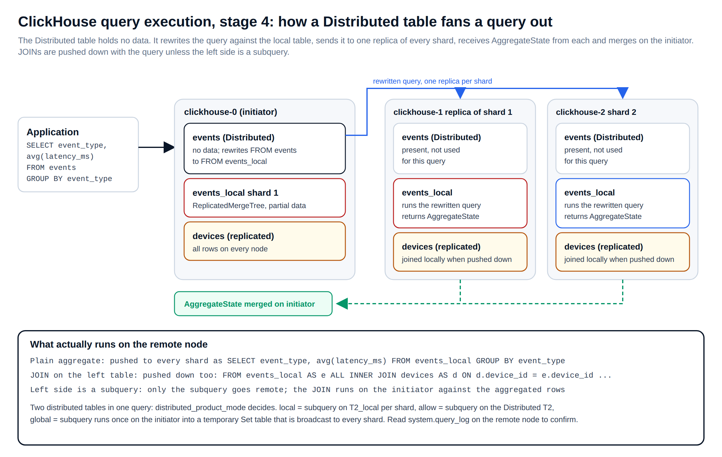
When the application queries events, distributed ClickHouse query execution begins on the initiator, which rewrites the innermost select against events_local and sends it to one replica of every shard. Each shard runs the query on its own parts and returns partial aggregate states, the same sum-and-count objects from stage 2, and the initiator merges them. The rewrite is literal:
-- What the application sends
SELECT event_type, avg(latency_ms) AS avg_latency
FROM telemetry.events
GROUP BY event_type ORDER BY avg_latency DESC;

-- What every shard actually runs
SELECT event_type, avg(latency_ms) AS avg_latency
FROM telemetry.events_local
GROUP BY event_type ORDER BY avg_latency DESC;
JOINs are pushed down by default
If the query joins the Distributed table to a replicated table, the JOIN goes to the shards along with everything else, which is exactly what you want when the right side exists on every node:
-- Sent by the application
SELECT e.device_id AS id, d.model AS m, count() AS c, avg(e.latency_ms) AS l
FROM telemetry.events e
JOIN telemetry.devices d ON d.device_id = e.device_id
GROUP BY id, m
HAVING c > 100000
ORDER BY l DESC
LIMIT 10;

-- Run on each shard
SELECT device_id AS id, model AS m, count() AS c, avg(latency_ms) AS l
FROM telemetry.events_local AS e
ALL INNER JOIN telemetry.devices AS d ON d.device_id = e.device_id
GROUP BY id, m
HAVING c > 100000
ORDER BY l DESC
LIMIT 10;
The exception in distributed ClickHouse query execution is the pattern from stage 3. When the left side is a subquery, only the subquery is sent to the remote servers; the JOIN then runs on the initiator against the rows that came back. That is often what you want for a small right side that is not replicated, and it is the same "aggregate first, then join" shape, just with the aggregation happening on the shards.
SELECT id, d.model, c AS events, l
FROM
(
    SELECT device_id AS id, count() AS c, avg(latency_ms) AS l
    FROM telemetry.events                      -- this part runs on the remote servers
    GROUP BY id
    HAVING c > 100000
    ORDER BY l DESC
) AS e
LEFT JOIN telemetry.devices d ON d.device_id = e.id   -- this part runs on the initiator
LIMIT 10;
Two distributed tables in one query: distributed_product_mode
ClickHouse query execution gets more complex when both tables in a query are distributed, for example SELECT … FROM events WHERE tenant_id IN (SELECT tenant_id FROM flagged_tenants) where both are Distributed. The setting distributed_product_mode decides what each shard sees. With local, the subquery is rewritten to the local table and runs against that shard's own slice, which is only correct if the two tables are sharded on the same key.
With allow, the subquery runs against the Distributed table on every shard, so each shard fans out again. With global, the subquery runs once on the initiator into a temporary table that is broadcast to every shard, and the outer query runs against the local table using that set.
-- distributed_product_mode = global, spelled out by hand
CREATE TEMPORARY TABLE flagged ENGINE = Set AS
SELECT tenant_id FROM telemetry.flagged_tenants;   -- runs once, on the initiator

SELECT count()
FROM telemetry.events_local
WHERE tenant_id IN flagged;                        -- runs on every shard with the set broadcast
Which mode is right for a given piece of ClickHouse query execution depends on where the data lives and how big the subquery result is, and there is no honest shortcut around thinking that through per query. The rules we apply are the same four every time: know where the data is located; move WHERE and heavy grouping work to the left-hand side of the join; use a subquery to order joins after the remote scan; and read system.query_log on the remote nodes to see what actually executed there, because the query the initiator logged is not the query the shard ran.
Checklist
The ClickHouse query execution checklist we leave with a team
Everything above collapses into one table. The left column is the stage, the middle column is what to look at, and the right column is what to change, in the order we would try it.
| Stage | Where to look | What to change, in order |
|---|---|---|
| INSERT | system.query_log for duration and memory; system.parts with level = 0 for part sizes | Batch bigger blocks; one partition key per block; then max_insert_threads and input_format_parallel_parsing, up for speed, down for memory |
| Storage | system.parts: rows, marks, compressed and uncompressed bytes per part | Large partitions and a part count in the hundreds; partition by month if unsure; a sort key that matches the filters |
| GROUP BY | memory_usage and read_rows per query in system.query_log | Lighter aggregate functions; fewer distinct key values; filter rows earlier; max_threads; spill with max_bytes_before_external_group_by as a last resort |
| JOIN | Right-side row count and column count; memory of the query | Aggregate in a subquery, then join; shrink and filter the right side; use a dictionary for shared lookups; remember IN is a join |
| Distributed | system.query_log on the remote nodes, not only the initiator | Replicate dimensions, shard facts; push WHERE and grouping left; subquery to join after the remote scan; set distributed_product_mode deliberately |
None of this is version-specific in spirit, but defaults and limits move between releases. Before applying a threshold or a setting to a production cluster, confirm it on your version, test it on a staging copy of your workload, and keep a rollback path. That caveat is not boilerplate; it is how we run ClickHouse query execution reviews for our own customers.
Where to read next
For more on ClickHouse query execution, the ClickHouse documentation covers MergeTree, Distributed tables and every setting named above, and the ClickHouse source is the final word when documentation and behaviour disagree. For the operational side of the same engine, see our guides on advanced ClickHouse troubleshooting and why ClickHouse is so fast.
ChistaDATA
When the model is clear and the query is still slow
ChistaDATA engineers run ClickHouse query execution reviews for production clusters across every stage in this article: ingestion batching and part sizing, aggregation memory, join placement and dictionary design, and distributed query planning across shards and replicas. Every recommendation arrives with the system.query_log evidence behind it and a rollback path. 24×7×365 support with S1 response in 15 minutes.
Running ClickHouse in production? ChistaDATA provides ClickHouse consulting for architecture, performance and migrations, and 24×7 ClickHouse support with a 15-minute S1 response. For day-to-day operations see ClickHouse DBA services and ClickHouse managed services.
