A ClickHouse JOIN is not chosen by a cost-based optimizer; it is chosen by the statement. The right-hand table is built into memory in whatever algorithm the session’s join_algorithm names, the left-hand table streams through it in the order written, and the engine does not reorder tables or pick a different algorithm because the statistics suggested one. That makes joins the one part of ClickHouse where the author’s decisions are the plan, and it is why the archive under this category reads like an algorithm reference rather than a tuning guide.
This page is that reference: six join algorithms with the memory model, the input each expects, the pipeline it produces and the case each is for; then the reasons inner joins on a column store cost what they do, chained joins, delta updates, and the four substitutes that remove a join altogether. The query performance hub covers the rewrite patterns around joins; this page covers the join itself.
The archive holds the internal mechanics of joins, hash joins in practice, nested-loop and merge-scan joins, why inner joins are expensive, chained joins, joins for real-time analytics, delta updates in OLAP, materialised view performance, and the 26.8 LTS settings that changed join defaults.
The model every ClickHouse JOIN shares: build right, probe left
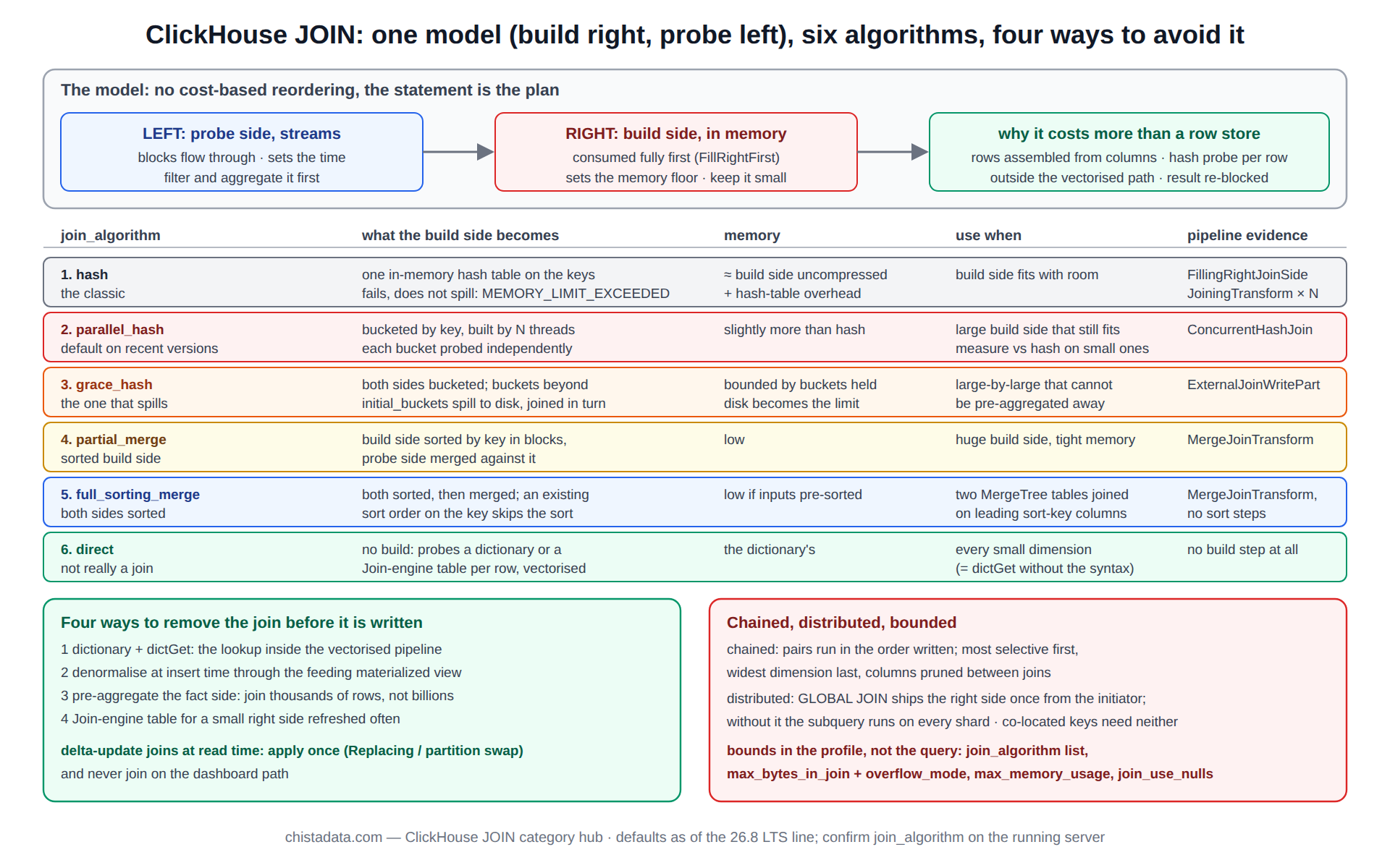
Whatever the algorithm, the right table is the build side and the left is the probe side. The build side is consumed completely before the first left row is processed (the pipeline shows it as FillRightFirst), so its size sets the memory floor, and the left side is streamed in blocks, so its size sets the time. Putting the fact table on the right is the single most expensive mistake in the category, and the internal mechanics of joins post explains why the engine does not save the author from it.
-- the shape to keep: small side right, big side left, filter and aggregate the big side first
SELECT c.plan, sum(e.amount) AS revenue
FROM
(
    SELECT customer_id, sum(amount) AS amount
    FROM events
    WHERE event_date >= today() - 30
    GROUP BY customer_id
) AS e
INNER JOIN customers AS c ON c.customer_id = e.customer_id
GROUP BY c.plan;

-- EXPLAIN PIPELINE shows the build side finishing first:
--   JoiningTransform × 8  ← probe
--   FillingRightJoinSide  ← build, customers
Algorithm 1: hash, the default ClickHouse JOIN and its memory bound
The build side is hashed into an in-memory table keyed by the join columns; each left block probes it. It is the fastest algorithm when the build side fits in memory and the reason max_memory_usage is the first setting a ClickHouse JOIN hits. Memory is roughly the build side’s uncompressed size plus hash-table overhead, and the query fails with MEMORY_LIMIT_EXCEEDED rather than spilling. The hash joins in ClickHouse post measures the overhead per row and per key type.
SET join_algorithm = 'hash';
-- memory the build side will take, before running the join
SELECT formatReadableSize(sum(data_uncompressed_bytes)) AS build_side_uncompressed
FROM system.columns WHERE table = 'customers';
-- after: ProfileEvents and peak memory in system.query_log for the join shape
SELECT formatReadableSize(memory_usage), ProfileEvents['JoinBuildTableRowCount'] AS build_rows
FROM system.query_log WHERE query_id = '${QUERY_ID}' AND type = 'QueryFinish';
Algorithm 2: parallel_hash, the same table built by many threads
parallel_hash splits the build side into buckets by key and builds them concurrently, then probes each bucket independently. It is faster than hash on large build sides at the cost of somewhat more memory, and it is the default on recent versions (the 26.8 LTS settings post records the switch). The choice between the two is measured, not assumed: on a small build side the bucketing overhead can cost more than it saves.
Algorithm 3: grace_hash, the ClickHouse JOIN that spills
When the build side does not fit, grace_hash partitions both sides by hash into buckets, keeps as many buckets in memory as grace_hash_join_initial_buckets allows, and spills the rest to disk, joining bucket by bucket. It trades time for a bounded memory footprint and is the algorithm for the occasional large-by-large join that cannot be pre-aggregated away. Disk throughput becomes the limit, and max_bytes_in_join still applies per bucket.
SET join_algorithm = 'grace_hash', grace_hash_join_initial_buckets = 16, max_bytes_in_join = 8000000000;
SELECT count() FROM big_left AS l JOIN big_right AS r ON l.k = r.k;
-- evidence: ProfileEvents['ExternalJoinWritePart'] and the temporary-data path fill during the query
Algorithms 4 and 5: partial_merge and full_sorting_merge, the sorted ClickHouse JOIN pair
partial_merge sorts the build side by key in blocks and merges the probe side against it, keeping memory low at the cost of sorting; full_sorting_merge sorts both sides and merges them, and can use an existing sort order on either side so that a join on the leading sort-key columns of two MergeTree tables skips the sort entirely.
Both are for inputs that are already ordered or far too large to hash, and both are slower than hash when hash fits. The nested loop and merge scan joins post walks the merge-scan mechanics and the pathological nested-loop case that a cross join or a non-equi condition produces.
-- two tables both sorted by (tenant_id, ts): the merge join reads them in order, no hash table
SET join_algorithm = 'full_sorting_merge';
SELECT count()
FROM events AS e
JOIN sessions AS s ON s.tenant_id = e.tenant_id AND s.ts = e.ts;
-- evidence: no FillingRightJoinSide in the pipeline; MergeJoinTransform instead
Algorithm 6: direct, the join that is a dictionary lookup
When the right side is a dictionary or a table with the Join engine, direct skips the build entirely and probes the existing structure per row inside the vectorised pipeline. It is the fastest ClickHouse JOIN there is, because it is not really a join, and it is the recommended form for every dimension small enough to hold in memory. dictGet in the select list is the same idea without the join syntax. The implementing joins for real-time analytics post builds a dashboard schema on this pattern.
CREATE DICTIONARY customer_dim
(
    customer_id UInt64,
    plan        String,
    region      String
)
PRIMARY KEY customer_id
SOURCE(CLICKHOUSE(table 'customers'))
LAYOUT(HASHED())
LIFETIME(MIN 300 MAX 600);

SET join_algorithm = 'direct';
SELECT d.plan, count()
FROM events AS e
JOIN dictionary('customer_dim') AS d ON d.customer_id = e.customer_id
WHERE e.event_date = today()
GROUP BY d.plan;
-- or, without join syntax at all:
SELECT dictGet('customer_dim', 'plan', customer_id) AS plan, count() FROM events WHERE event_date = today() GROUP BY plan;| Algorithm | Build side | Memory | Best for | Evidence in the pipeline |
|---|---|---|---|---|
| hash | hashed in memory | ≈ build side uncompressed + overhead | build side fits comfortably | FillingRightJoinSide, JoiningTransform |
| parallel_hash | bucketed, built by N threads | slightly more than hash | large build side that still fits | ConcurrentHashJoin transforms |
| grace_hash | bucketed, buckets spill to disk | bounded by buckets in memory | large-by-large, cannot pre-aggregate | ExternalJoinWritePart events |
| partial_merge | sorted in blocks | low | huge build side, memory-tight | MergeJoinTransform, sort steps |
| full_sorting_merge | both sides sorted | low if inputs pre-sorted | both sides ordered by the key | MergeJoinTransform, no sort if ordered |
| direct | none: dictionary or Join engine | the dictionary’s | every small dimension | no build step at all |
Why an inner ClickHouse JOIN costs more than it would in a row store
Three reasons, all consequences of the column store. The build side must be materialised as rows from columns, which is the decompression and assembly a column store otherwise avoids. The probe runs a hash lookup per row outside the vectorised fast path that filters and aggregates run in. And the result must be re-assembled into blocks before the next operator, which is a copy. None of this is a defect; it is the price of joining in a system built to avoid joining, and the why are inner joins expensive post measures each of the three on a benchmark table.
Chained ClickHouse JOIN order and intermediate size
A query with three ClickHouse JOIN clauses is three build-probe pairs in the order written, and the intermediate result of each becomes the probe side of the next, so the order decides how large the intermediates are. The rule is to join the most selective pair first and the widest dimension last, with each intermediate as narrow as possible (select only the columns the next join and the final projection need). The mastering chained joins post works through the reordering with plan evidence, and the EXPLAIN hub shows how to read the build sides off the pipeline.
-- chained: most selective first, columns pruned between joins
SELECT r.region, p.plan, count()
FROM
(
    SELECT e.customer_id, e.amount
    FROM events AS e
    WHERE e.event_date = today() AND e.event_type = 'purchase'      -- selective filter before any join
) AS e
JOIN customers AS c ON c.customer_id = e.customer_id                  -- 50k rows: small build
JOIN plans     AS p ON p.plan_id     = c.plan_id                      -- 20 rows
JOIN regions   AS r ON r.region_id   = c.region_id                    -- 12 rows
GROUP BY r.region, p.plan;
The four substitutes that remove a ClickHouse JOIN
Most ClickHouse JOIN statements in analytical queries are lookups of slowly changing attributes, and four techniques replace them: a dictionary with dictGet (algorithm 6 without the syntax); denormalising the attribute into the fact table at insert time, usually through the materialised view that feeds it; pre-aggregating the fact side so the join runs over thousands of rows rather than billions; and a Join engine table for a right side that must be refreshed often but is small. The materialized view performance post covers the denormalising view, and the machine learning hub shows the substitutes applied to feature queries.
-- substitute 2: denormalise at insert time through the feeding view
CREATE MATERIALIZED VIEW events_mv TO events AS
SELECT
    k.ts, k.customer_id, k.amount,
    dictGet('customer_dim', 'plan',   k.customer_id) AS plan,
    dictGet('customer_dim', 'region', k.customer_id) AS region
FROM events_kafka AS k;
-- the dashboard query then has no join at all: GROUP BY plan, region over events
Delta updates and the join that should not exist
A recurring anti-pattern joins a fact table to a “changes” table to apply corrections at read time: every query re-applies the deltas, which is a join over the largest table in the system on every dashboard refresh. The delta updates in OLAP databases post explains why the cost compounds and what to do instead: apply the deltas once through a ReplacingMergeTree version or a partition swap, both covered on the updates hub, so that reads never join.
Distributed joins: GLOBAL and where the build side goes
On a sharded cluster a ClickHouse JOIN runs on every shard, and without GLOBAL each shard evaluates the right side independently, which for a subquery means re-running it once per shard. GLOBAL JOIN evaluates the right side once on the initiator and ships it to every shard as a temporary table, so the right side must be small enough to ship. When both sides are large and sharded by the same key, the join is correct shard-locally and GLOBAL is unnecessary; when they are not co-located, the query is usually redesigned rather than joined. The sharding hub covers co-location.
SET distributed_product_mode = 'global';
SELECT count()
FROM events_dist AS e
GLOBAL JOIN (SELECT customer_id FROM customers WHERE plan = 'enterprise') AS c ON c.customer_id = e.customer_id;
-- shipped once from the initiator; without GLOBAL the subquery runs on every shard
Settings that bound a ClickHouse JOIN
Four settings decide what a join may cost: join_algorithm (which of the six, or a list the engine tries in order), max_bytes_in_join and max_rows_in_join with join_overflow_mode (fail or truncate when the build side exceeds them), max_memory_usage as the outer bound, and join_use_nulls which changes the semantics of outer joins from default values to NULL. They belong in the settings profile of each client class, not in individual queries, and the memory hub covers where join memory sits among the other consumers.
CREATE SETTINGS PROFILE analyst_profile SETTINGS
    join_algorithm     = 'parallel_hash,grace_hash',   -- try in order
    max_bytes_in_join  = 4000000000,
    join_overflow_mode = 'throw',
    max_memory_usage   = 32000000000,
    join_use_nulls     = 1;

-- what each join shape actually cost, last day
SELECT normalized_query_hash, count() AS runs, formatReadableSize(max(memory_usage)) AS peak, quantile(0.95)(query_duration_ms) AS p95
FROM system.query_log
WHERE type = 'QueryFinish' AND query ILIKE '%JOIN%' AND event_time > now() - INTERVAL 1 DAY
GROUP BY normalized_query_hash ORDER BY max(memory_usage) DESC LIMIT 10;
ASOF and semi joins: the two shapes that are not lookups
Two join kinds deserve their own mention because they replace patterns that are otherwise self-joins. ASOF JOIN matches each left row to the nearest right row on an inequality (the latest price at or before a trade time, the session active when an event happened), which a row store would express as a correlated subquery and a column store cannot afford; it runs as a hash join whose build side is sorted per key.
SEMI and ANTI joins answer “exists” and “does not exist” without producing duplicate rows, and are the correct form for the IN (subquery) shapes that grow past the size an IN set handles well.
-- latest quote at or before each trade: one ASOF JOIN instead of a correlated subquery
SELECT t.trade_id, t.ts, q.price
FROM trades AS t
ASOF LEFT JOIN quotes AS q ON q.symbol = t.symbol AND q.ts <= t.ts;

-- customers with no purchase this month, without duplicates or a large IN set
SELECT c.customer_id
FROM customers AS c
ANTI JOIN (SELECT customer_id FROM events WHERE event_type = 'purchase' AND event_date >= toStartOfMonth(today())) AS p
    ON p.customer_id = c.customer_id;
Both shapes keep the build-right model: the quotes table and the purchase subquery are the build sides above, and the same memory arithmetic applies. An ASOF build side that holds a year of quotes for every symbol is as expensive as any other large build side, and is trimmed to the time window the left side spans before the join runs.
Version notes
grace_hash is 22.x and later; full_sorting_merge 22.x; direct with dictionaries 21.x; parallel_hash as the default on the 24.x and later line, with the exact release recorded in the 26.8 settings post. join_algorithm accepts a comma-separated list on recent versions and tries each in order. The JOIN clause documentation is the source for the algorithms and settings above; confirm the default on the running version.
Reading the archive
The archive was written across 23.x to 26.8, so the algorithm defaults quoted in the older posts differ from current ones; the settings post is the authority for what the running version does.
Start with the internal mechanics post for the model, then hash joins and nested-loop-and-merge-scan for the algorithms, why inner joins are expensive for the cost, chained joins for order, and the real-time analytics post for the dictionary pattern in a schema. Delta updates and materialized view performance cover the two ways a join should have been removed before it was written.
ChistaDATA reviews every join shape in the query log during a ClickHouse consulting performance review, records the build-side size and memory per shape, and keeps the profiles bounded under 24×7 support. Every algorithm change and every substitute on this page is tested on staging against a production-sized sample, with parity of results checked before speed.