ClickHouse analytics platforms fail or succeed on decisions made before the first query is written: how events enter the cluster, what the sort key of the fact table is, whether dashboards read raw rows or pre-aggregated targets, and which numbers are watched once the platform is live. The engine itself is rarely the bottleneck; the arrangement around it is.
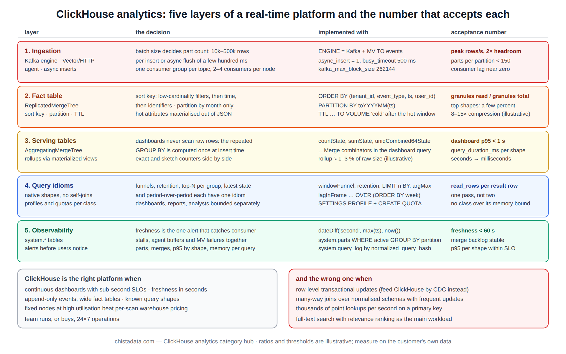
This page lays out a real-time analytics platform as five layers, from ingestion to observability, with the decision that matters at each layer, the SQL that implements it, and the archive post that goes deeper. It also covers the cases where ClickHouse is the wrong choice, because a platform review that cannot say no is not a review.
The archive under this category spans reference architectures for retail and telecom, platform comparisons against Snowflake and BigQuery, the batch-to-real-time transition, SQL techniques such as window functions and conditional analysis, and operational posts on hot spots and observability pipelines.
What ClickHouse analytics means in practice
“Real-time analytics” is used loosely; on this page it means a fixed set of measurable properties. Events are queryable within seconds of being produced (freshness). Queries over the last hour, day and month return in under a second at p95 for the dashboard shapes (latency). The platform sustains the peak ingestion rate with headroom, typically hundreds of thousands to millions of rows per second per node (throughput). Concurrency is bounded and predictable, usually tens to low hundreds of concurrent dashboard queries rather than thousands of point lookups.
Those four numbers, freshness, latency, throughput and concurrency, are the acceptance criteria for every layer below. The real-time analytics architecture post sets them out as a reference design; the batch to real-time post describes the transition for a platform that started on nightly loads.
Layer 1: ingestion for ClickHouse analytics at event rate
The first decision is how events reach the cluster. Three paths cover most platforms: a Kafka topic consumed by the Kafka table engine or ClickPipes-style consumer, a Vector or Fluent Bit agent posting batches over HTTP, or an application writing directly with async inserts. Each has a distinct failure mode: consumer lag, agent buffer overflow, and part explosion from small synchronous inserts.
The rule that holds across all three is batch size. ClickHouse creates one part per insert, and merges are the cost of small parts; inserts of 10,000 to 500,000 rows, or async inserts with a flush window of a few hundred milliseconds, keep system.parts healthy. The connecting ClickHouse to Kafka post walks through the engine path and the Vector pipeline post through the agent path.
-- Kafka path: engine table + materialized view into the fact table
CREATE TABLE events_kafka
(
    ts          DateTime64(3),
    tenant_id   UInt32,
    event_type  LowCardinality(String),
    user_id     UInt64,
    amount      Decimal(18, 2),
    attrs       String
)
ENGINE = Kafka
SETTINGS kafka_broker_list = '${KAFKA_BROKERS}',
         kafka_topic_list  = 'events',
         kafka_group_name  = 'clickhouse_events_v1',
         kafka_format      = 'JSONEachRow',
         kafka_num_consumers = 4,
         kafka_max_block_size = 262144;

CREATE MATERIALIZED VIEW events_kafka_mv TO events AS
SELECT ts, tenant_id, event_type, user_id, amount, attrs
FROM events_kafka;

-- direct path: async inserts, server-side batching
SET async_insert = 1, wait_for_async_insert = 1, async_insert_busy_timeout_ms = 500;
Layer 2: the fact table and its sort key
Every analytical query pays for the bytes it reads, and the sort key decides how many bytes a typical predicate leaves. The order is low-cardinality filters first, then the time column, then high-cardinality identifiers; a key that starts with the timestamp prunes well for time-range queries and badly for tenant-scoped ones, which is the wrong way round for most ClickHouse analytics workloads where every dashboard is filtered by tenant, region or product first.
Partitioning is monthly or daily by the time column and nothing else. Partition by tenant looks attractive and produces thousands of small parts. The hot spot detection post covers the shard-level version of the same mistake, where one tenant’s traffic lands on one node.
CREATE TABLE events
(
    ts          DateTime64(3)          CODEC(Delta, ZSTD(1)),
    tenant_id   UInt32,
    event_type  LowCardinality(String),
    user_id     UInt64,
    amount      Decimal(18, 2),
    attrs       String                 CODEC(ZSTD(3)),
    event_date  Date MATERIALIZED toDate(ts)
)
ENGINE = ReplicatedMergeTree('/clickhouse/tables/{shard}/events', '{replica}')
PARTITION BY toYYYYMM(ts)
ORDER BY (tenant_id, event_type, ts, user_id)
TTL toDateTime(ts) + INTERVAL 13 MONTH TO VOLUME 'cold'
SETTINGS index_granularity = 8192;
Layer 3: serving tables, because ClickHouse analytics dashboards should not scan raw rows
A dashboard that refreshes every 30 seconds and runs the same GROUP BY over a day of raw events is the most common source of load on a ClickHouse analytics cluster. The fix is to compute the aggregate once at insert time into an AggregatingMergeTree or SummingMergeTree target through a materialized view, and point the dashboard at the target. Queries move from seconds to milliseconds and the cost moves to the insert path, where it is paid once.
The materialized view hub covers topology and pitfalls in depth; the pattern below is the minimum shape for a per-minute rollup with exact and approximate counters side by side.
CREATE TABLE events_1m
(
    minute      DateTime,
    tenant_id   UInt32,
    event_type  LowCardinality(String),
    events      AggregateFunction(count),
    revenue     AggregateFunction(sum, Decimal(18, 2)),
    users       AggregateFunction(uniqCombined64, UInt64)
)
ENGINE = ReplicatedAggregatingMergeTree('/clickhouse/tables/{shard}/events_1m', '{replica}')
PARTITION BY toYYYYMM(minute)
ORDER BY (tenant_id, event_type, minute);

CREATE MATERIALIZED VIEW events_1m_mv TO events_1m AS
SELECT
    toStartOfMinute(ts)              AS minute,
    tenant_id,
    event_type,
    countState()                     AS events,
    sumState(amount)                 AS revenue,
    uniqCombined64State(user_id)     AS users
FROM events
GROUP BY minute, tenant_id, event_type;

-- dashboard query: milliseconds, reads the rollup only
SELECT minute, countMerge(events), sumMerge(revenue), uniqCombined64Merge(users)
FROM events_1m
WHERE tenant_id = 42 AND minute >= now() - INTERVAL 1 DAY
GROUP BY minute ORDER BY minute;
Layer 4: the SQL that ClickHouse analytics teams actually write
Most analytical questions are one of a handful of shapes: time-bucketed aggregates, funnels and retention, top-N per group, sessionisation, and comparisons across periods. ClickHouse has native idioms for each that avoid self-joins: windowFunnel and retention for funnels, LIMIT n BY group for top-N, argMax for latest-state, and window functions since 21.x for running totals and period-over-period.
The window functions with OVER post covers the frame semantics, the conditional analysis post the -If combinators, and the finding missing values post the anti-join and set techniques for reconciliation.
-- week-over-week revenue with a window, no self-join
SELECT
    week,
    revenue,
    revenue - lagInFrame(revenue, 1) OVER (ORDER BY week)                 AS wow_delta,
    round(100 * revenue / lagInFrame(revenue, 1) OVER (ORDER BY week) - 100, 1) AS wow_pct
FROM
(
    SELECT toStartOfWeek(minute) AS week, sumMerge(revenue) AS revenue
    FROM events_1m
    WHERE tenant_id = 42 AND minute >= now() - INTERVAL 12 WEEK
    GROUP BY week
)
ORDER BY week;

-- conversion funnel in one pass
SELECT
    countIf(level >= 1) AS viewed,
    countIf(level >= 2) AS added,
    countIf(level >= 3) AS purchased
FROM
(
    SELECT user_id,
           windowFunnel(1800)(ts, event_type = 'view', event_type = 'add_to_cart', event_type = 'purchase') AS level
    FROM events
    WHERE tenant_id = 42 AND event_date = today()
    GROUP BY user_id
);
Layer 5: observability for the platform itself
A ClickHouse analytics platform needs its own dashboards before it serves anyone else’s: ingestion lag per topic or agent, parts per partition, merge backlog, query p95 by normalized shape, and memory per query. All of it is in system.* tables, and the monitoring hub sets out the twelve metrics that matter with alert thresholds.
The single most useful alert on a real-time platform is freshness: the age of the newest row in the fact table compared with wall-clock time. It catches consumer stalls, agent buffer problems and materialized-view failures in one number.
-- freshness: seconds between now and the newest event, per tenant class
SELECT
    tenant_id % 8                                   AS tenant_bucket,
    dateDiff('second', max(ts), now())              AS lag_s
FROM events
WHERE event_date >= today() - 1
GROUP BY tenant_bucket
HAVING lag_s > 60
ORDER BY lag_s DESC;

-- parts pressure: the number that precedes TOO_MANY_PARTS
SELECT database, table, partition, count() AS parts, sum(rows) AS rows
FROM system.parts
WHERE active
GROUP BY database, table, partition
HAVING parts > 150
ORDER BY parts DESC;
ClickHouse analytics versus Snowflake and BigQuery: where the cost goes
The platform comparison is a workload question, not a feature list. Cloud warehouses charge for compute time or bytes scanned, so a dashboard that refreshes every 30 seconds and scans a day of events is priced per refresh; ClickHouse on fixed nodes prices the same dashboard at the cost of the nodes, which is why the break-even moves quickly in ClickHouse’s favour as query frequency rises. The reverse holds for infrequent, very large ad hoc scans over cold data, where a warehouse’s elastic compute is cheaper than idle nodes.
The ClickHouse versus Snowflake post and the Snowflake versus BigQuery versus ClickHouse post work through the cost models with illustrative workloads. The migration posts under the columnar databases hub cover the move once the decision is made.
| Workload property | Favours ClickHouse | Favours a cloud warehouse |
|---|---|---|
| Query frequency | continuous dashboards, sub-second SLOs | occasional analyst sessions |
| Freshness need | seconds | hourly or daily loads acceptable |
| Data shape | append-only events, wide fact tables | heavy multi-table joins, frequent updates |
| Concurrency | tens to hundreds of known shapes | many ad hoc, unpredictable queries |
| Operations | team can run or buy 24×7 operations | no operations capacity at all |
| Cost model | fixed nodes, high utilisation | elastic, bursty, low utilisation |
When ClickHouse is the wrong platform
ChistaDATA sells ClickHouse services and still recommends against it for several workload classes. Transactional updates at row level (order status changing ten times) belong in PostgreSQL or MySQL with ClickHouse fed by CDC. Workloads dominated by many-way joins across normalised schemas with frequent updates are better served by a warehouse or an HTAP engine. Point lookups at thousands per second on a primary key are a key-value or OLTP job. Full-text search with relevance ranking belongs in a search engine, with ClickHouse holding the analytics on the same events.
Recognising these early is cheaper than migrating out later, and the columnar versus row-based post sets out the storage-level reason each class behaves as it does.
Reference architectures in the archive: retail, telecom, payments
Three archive posts apply the five layers to a domain. The retail analytics with Python post builds the ingestion and serving layers for order and inventory events with a Python producer and a dashboard reader. The real-time analytics for telcos post covers CDR and network-event volumes, where throughput dominates and the sort key is subscriber-first. The achieving real-time analytics post is the earliest statement of the design and still holds.
The ChistaDATA Cloud architecture post describes how the same layers are packaged as a managed platform, with Keeper, object-storage tiering and per-tenant quotas already in place.
Benchmarking a ClickHouse analytics platform honestly
Benchmarks that matter are run with the customer’s own top query shapes against a production-sized sample, not with a generic suite. TPC-DS is still useful as a regression harness across versions and hardware, because the queries are fixed and the results comparable over time; the TPC-DS benchmarking setup post covers data generation, loading and the schema adaptations ClickHouse needs.
Whichever suite is used, the same discipline applies: warm the cache or drop it deliberately, run each shape at least five times, report p50 and p95 rather than the best run, and record read_rows, read_bytes and memory_usage from system.query_log alongside the timing so that a regression can be attributed rather than guessed at.
-- benchmark harvest: one row per shape, from the query log, after a run tagged by log_comment
SELECT
    normalized_query_hash                       AS shape,
    count()                                     AS runs,
    quantile(0.5)(query_duration_ms)            AS p50_ms,
    quantile(0.95)(query_duration_ms)           AS p95_ms,
    formatReadableQuantity(avg(read_rows))      AS read_rows,
    formatReadableSize(avg(read_bytes))         AS read_bytes,
    formatReadableSize(max(memory_usage))       AS peak_mem,
    any(substring(query, 1, 80))                AS sample
FROM system.query_log
WHERE type = 'QueryFinish'
  AND log_comment = 'bench:2026-09-19:26.8'
GROUP BY shape
ORDER BY p95_ms DESC;
Nested and semi-structured data in ClickHouse analytics
Event payloads carry attributes that change per event type, and the choice between a String holding JSON, Map(String, String), typed Nested columns and the JSON type (production-ready since 25.x) decides whether attribute filters use an index or parse every row. The rule is to materialise the attributes that appear in predicates as real columns and leave the long tail in a Map or JSON column.
The application domain index for nested data post shows the materialised-column and skip-index pattern for the attributes that matter; the index hub covers the skip-index types themselves.
-- promote a hot attribute out of the JSON payload, then index it
ALTER TABLE events
    ADD COLUMN campaign_id LowCardinality(String)
        MATERIALIZED JSONExtractString(attrs, 'campaign_id');

ALTER TABLE events
    ADD INDEX idx_campaign campaign_id TYPE bloom_filter(0.01) GRANULARITY 4;

ALTER TABLE events MATERIALIZE COLUMN campaign_id IN PARTITION 202609;
ALTER TABLE events MATERIALIZE INDEX  idx_campaign IN PARTITION 202609;
Capacity and cost per layer
Sizing follows the layers. Ingestion nodes are sized by peak rows per second with 2× headroom; storage by compressed bytes per day multiplied by retention, with a 30 percent margin for merges; serving by the concurrent query count multiplied by the per-query memory bound. Object-storage tiering after the hot window (typically 30 to 90 days) is where most of the cost saving comes from on a mature platform, and the horizontal scaling hub covers the shard and replica arithmetic once one node is not enough.
Illustrative ratios from platforms of this shape: 8 to 15× compression on event data with ZSTD and Delta codecs, 200,000 to 800,000 rows per second per node sustained ingestion, and rollup tables at 1 to 3 percent of the raw table size. Actual figures depend on the schema and must be measured on the customer’s data.
Concurrency control on a shared ClickHouse analytics cluster
A platform that serves dashboards, scheduled reports and analysts from one cluster needs the three classes kept apart, or one analyst’s 40 GB join takes the dashboards down with it. Settings profiles bound each class by memory, rows and threads; quotas bound query counts per interval; and max_concurrent_queries_for_user stops a single integration from saturating the pool. The bounds are set from the query log, at roughly twice the observed p99 for each class, and reviewed monthly.
CREATE SETTINGS PROFILE dashboard_profile SETTINGS
    max_execution_time = 10,
    max_memory_usage   = 4000000000,
    max_threads        = 8,
    max_result_rows    = 100000;

CREATE SETTINGS PROFILE analyst_profile SETTINGS
    max_execution_time = 300,
    max_memory_usage   = 32000000000,
    max_bytes_before_external_group_by = 16000000000,
    max_threads        = 16;

CREATE QUOTA analyst_quota
    FOR INTERVAL 1 HOUR MAX queries = 500, read_bytes = 2000000000000
    TO analyst_role;

ALTER USER ${CH_DASHBOARD_USER} SETTINGS PROFILE 'dashboard_profile';
ALTER USER ${CH_DASHBOARD_USER} SETTINGS max_concurrent_queries_for_user = 40;
Version notes
Window functions are 21.x and later; async_insert stable since 22.x; uniqCombined64 and windowFunnel have been available since 20.x. The JSON type is production-ready since 25.x and replaces the earlier Object('json'); on 24.x and earlier keep JSON in a String with materialised columns. Kafka engine settings named above are current as of 24.x and later. The Kafka table engine documentation is the source for consumer settings; confirm behaviour on the running version.
Reading the archive
Read by layer. For ingestion: connecting to Kafka, the Vector pipeline, and batch to real-time. For the fact table and hot spots: hot spot detection and remediation, and the columnar versus row-based post. For serving and SQL: window functions, conditional analysis, and missing values. For platform choice and cost: ClickHouse versus Snowflake, and the three-way cost comparison. For domain designs: retail, telco, and the ChistaDATA Cloud architecture. For measurement: TPC-DS setup.
ChistaDATA designs and operates ClickHouse analytics platforms through ClickHouse consulting and runs them under managed services with the freshness, latency and parts alerts above in place from day one. Every design on this page should be tested on staging with production-shaped data before it is applied to a running cluster, with a tested backup and restore path in place.