Time-series analytics in ClickHouse comes down to five schema decisions made before the first row lands: the sort key, the partition and TTL scheme, the column codecs, the rollup topology, and the query functions the application will lean on. Get those five right and a single MergeTree table serves metrics, logs, traces, IoT telemetry and market ticks at billions of rows per day with sub-second dashboards. Get one wrong and the table works fine for a month, then merges fall behind, storage doubles, and every query does a full scan. This page is our reference for those five decisions, with the DDL we actually deploy, the queries that verify each choice, and the anti-patterns we are called in to fix.
It sits above the archive’s introductory post, Time-series analytics at scale with ClickHouse, which explains why a general-purpose columnar engine has become the default for this workload. This page assumes that case is made and goes into the engineering.
Decision 1: the time-series analytics sort key follows query selectivity, not time
The most common time-series analytics mistake in ClickHouse is ORDER BY (timestamp). Time is the least selective column in almost every query: a dashboard asks for the last hour across one service, one host, or one tenant, and a timestamp-first key forces the engine to scan every series for that hour. The sort key should begin with the columns that narrow the series set, in increasing cardinality order, and end with time.
CREATE TABLE metrics
(
    ts         DateTime64(3, 'UTC')  CODEC(DoubleDelta, ZSTD(1)),
    tenant_id  UInt32                CODEC(ZSTD(1)),
    service    LowCardinality(String),
    host       LowCardinality(String),
    metric     LowCardinality(String),
    labels     Map(LowCardinality(String), String) CODEC(ZSTD(3)),
    value      Float64               CODEC(Gorilla, ZSTD(1))
)
ENGINE = ReplicatedMergeTree('/clickhouse/tables/{shard}/metrics', '{replica}')
PARTITION BY toYYYYMMDD(ts)
ORDER BY (tenant_id, service, metric, host, ts)
TTL toDateTime(ts) + INTERVAL 14 DAY
SETTINGS index_granularity = 8192;
Confirm the key is doing its job by checking how many granules a representative query reads relative to the table:
EXPLAIN indexes = 1
SELECT toStartOfMinute(ts) AS m, avg(value)
FROM metrics
WHERE tenant_id = 42
  AND service = 'checkout'
  AND metric = 'http_request_duration_p95'
  AND ts >= now() - INTERVAL 1 HOUR
GROUP BY m
ORDER BY m;

-- look for:  PrimaryKey  Parts: 3/48  Granules: 12/91234
If Granules shows a small numerator over a large denominator the key matches the workload. If it shows most granules selected, the leading key columns are not in the predicate and the key needs reordering, or a projection with a different order is needed for that query family.
Cardinality matters at the tail of the key too. Putting a high-cardinality host before metric when queries filter on metric first destroys locality; the order above assumes queries name the metric more often than the host. Read the predicate profile from system.query_log before deciding, not the schema.
Decision 2: partition by the retention unit and let TTL do the deletes
Partitions in a ClickHouse time-series analytics table are for lifecycle, not for query pruning; the primary index handles pruning. A daily partition for a 14-day table gives roughly fourteen active partitions, a bounded part count, and cheap TTL deletes that drop whole parts rather than rewriting them. Monthly partitions on a two-week retention would leave a rolling rewrite of the oldest partition every day; hourly partitions on a one-year retention would create thousands of partitions and starve the merge scheduler.
The rule we apply: choose the partition unit so that the table holds between ten and a few hundred active partitions, and align the TTL to a whole number of that unit. Verify with:
SELECT
    partition,
    count()                                AS parts,
    sum(rows)                              AS rows,
    formatReadableSize(sum(bytes_on_disk)) AS on_disk,
    min(min_time)                          AS oldest,
    max(max_time)                          AS newest
FROM system.parts
WHERE database = currentDatabase()
  AND table = 'metrics'
  AND active
GROUP BY partition
ORDER BY partition DESC;
More than a few dozen parts per partition in steady state points at insert batches that are too small, and the fix is upstream in the ingestion layer (batching, async_insert), not in the schema. Tiered TTL, moving parts older than a few days to an object-storage volume, keeps the NVMe footprint to the hot window; the storage-policy pattern for that is on our baremetal ClickHouse page.
Decision 3: codecs turn time-series analytics into a compression problem you can win
Time-series columns are unusually compressible because consecutive values are correlated. ClickHouse exposes specialized codecs that exploit exactly this, and choosing them per column is where a 10x storage difference lives.
| Column shape | Codec | Why |
|---|---|---|
| Monotonic timestamps at a regular interval | DoubleDelta, ZSTD(1) | Second-order deltas of a regular series are near-zero and compress to bits |
| Timestamps at irregular intervals | Delta, ZSTD(1) | First-order deltas remain small; DoubleDelta gains nothing |
| Gauge floats (temperature, latency, price) | Gorilla, ZSTD(1) | XOR of consecutive floats has short mantissa differences |
| Monotonic counters (bytes sent, request totals) | Delta, ZSTD(1) on the integer form | Deltas are small positive integers |
| Integers with a bounded range (status codes, small IDs) | T64, ZSTD(1) | Transposes 64-bit blocks so unused high bits vanish |
| Low-cardinality strings | LowCardinality(String) type, default codec | Dictionary encoding does the work before any codec runs |
| Free-form labels, JSON | ZSTD(3) | General-purpose; higher level pays off on text |
Measure rather than assume. The per-column compression ratio is in system.columns, and comparing two codec choices on a copy of a day’s partition takes minutes:
SELECT
    name,
    compression_codec,
    formatReadableSize(data_uncompressed_bytes) AS raw,
    formatReadableSize(data_compressed_bytes)   AS compressed,
    round(data_uncompressed_bytes / data_compressed_bytes, 1) AS ratio
FROM system.columns
WHERE database = currentDatabase()
  AND table = 'metrics'
ORDER BY data_compressed_bytes DESC;
Ratios above 20 on the timestamp column and above 5 on gauge values are normal for regular telemetry with the codecs above. A timestamp column under 5x is a sign that the series interleave badly within a granule, which loops back to Decision 1: the sort key groups series so that consecutive rows belong to the same series and the deltas are regular.
Decision 4: time-series analytics rollups as materialized views into AggregatingMergeTree
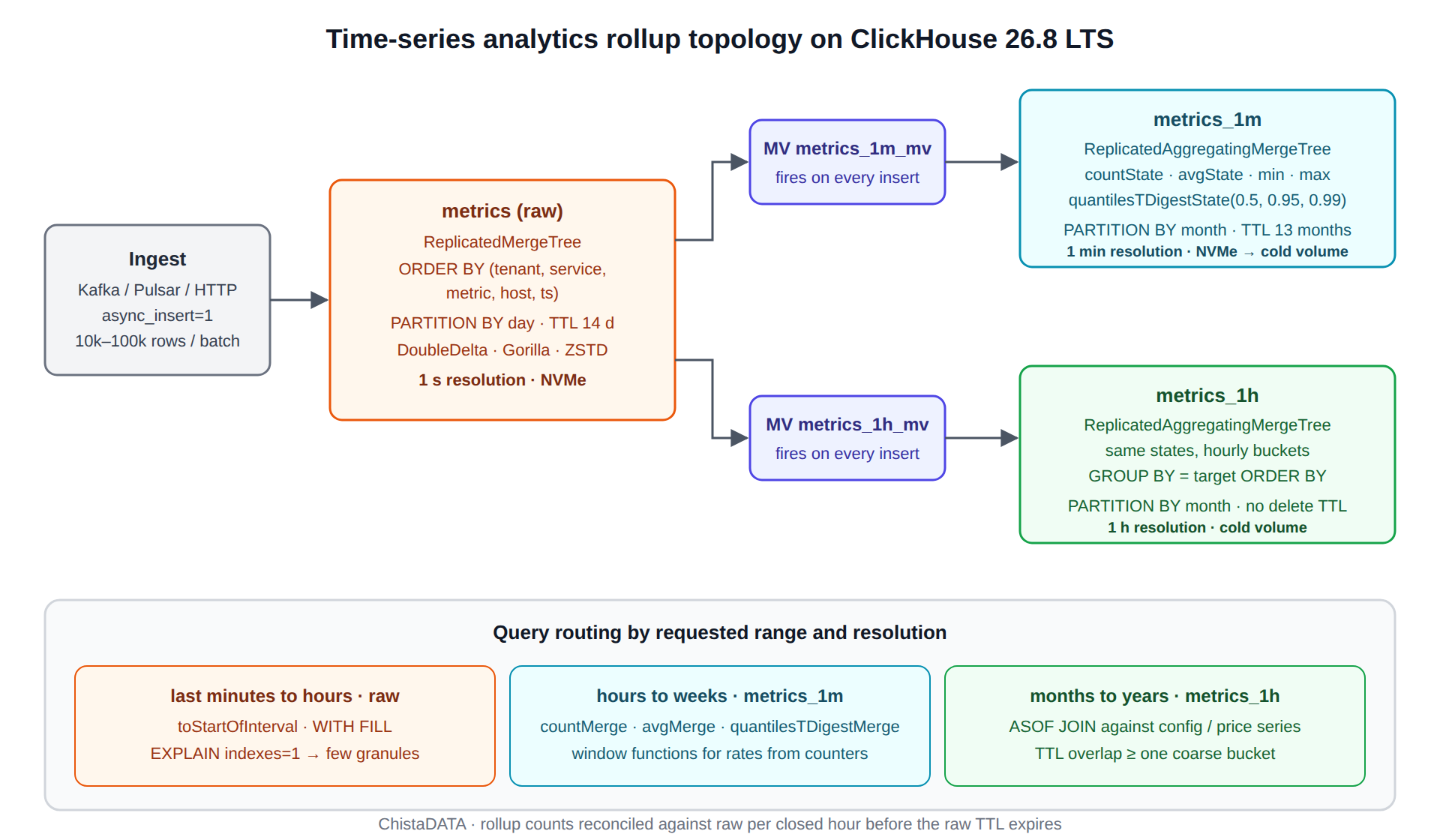
Time-series analytics dashboards do not read raw one-second samples for a thirty-day chart; they read a per-minute or per-hour rollup. In ClickHouse the rollup is a materialized view that fires on every insert into the raw table and writes aggregate states into an AggregatingMergeTree target. The states merge correctly across parts, which is why -State and -Merge combinators are used rather than plain aggregates.
CREATE TABLE metrics_1m
(
    ts_min     DateTime('UTC')       CODEC(DoubleDelta, ZSTD(1)),
    tenant_id  UInt32,
    service    LowCardinality(String),
    metric     LowCardinality(String),
    host       LowCardinality(String),
    samples    AggregateFunction(count),
    v_avg      AggregateFunction(avg, Float64),
    v_min      SimpleAggregateFunction(min, Float64),
    v_max      SimpleAggregateFunction(max, Float64),
    v_q        AggregateFunction(quantilesTDigest(0.5, 0.95, 0.99), Float64)
)
ENGINE = ReplicatedAggregatingMergeTree('/clickhouse/tables/{shard}/metrics_1m', '{replica}')
PARTITION BY toYYYYMM(ts_min)
ORDER BY (tenant_id, service, metric, host, ts_min)
TTL ts_min + INTERVAL 13 MONTH;

CREATE MATERIALIZED VIEW metrics_1m_mv TO metrics_1m AS
SELECT
    toStartOfMinute(ts)                                    AS ts_min,
    tenant_id,
    service,
    metric,
    host,
    countState()                                           AS samples,
    avgState(value)                                        AS v_avg,
    min(value)                                             AS v_min,
    max(value)                                             AS v_max,
    quantilesTDigestState(0.5, 0.95, 0.99)(value)          AS v_q
FROM metrics
GROUP BY ts_min, tenant_id, service, metric, host;

-- reading the rollup
SELECT
    ts_min,
    countMerge(samples)                        AS n,
    avgMerge(v_avg)                            AS avg_v,
    max(v_max)                                 AS max_v,
    quantilesTDigestMerge(0.5, 0.95, 0.99)(v_q) AS q
FROM metrics_1m
WHERE tenant_id = 42
  AND service = 'checkout'
  AND metric = 'http_request_duration_p95'
  AND ts_min >= now() - INTERVAL 24 HOUR
GROUP BY ts_min
ORDER BY ts_min;
Two rules keep this topology healthy. The materialized view’s GROUP BY must match the target table’s ORDER BY exactly so that states for the same bucket collapse on merge. And the raw table’s TTL must be longer than the maximum ingestion delay, because a materialized view only sees rows at insert time; late data arriving after the raw row would have expired still lands, but any rollup it should have joined is already a separate state row, which the -Merge read handles correctly. Verify the rollup is complete by comparing counts for a closed hour:
SELECT
    (SELECT count() FROM metrics
      WHERE tenant_id = 42 AND ts >= '2026-09-17 10:00:00' AND ts < '2026-09-17 11:00:00') AS raw_rows,
    (SELECT countMerge(samples) FROM metrics_1m
      WHERE tenant_id = 42 AND ts_min >= '2026-09-17 10:00:00' AND ts_min < '2026-09-17 11:00:00') AS rollup_rows;
Decision 5: the query functions that define time-series analytics in ClickHouse
Application code should lean on the functions built for this workload rather than emulating them with self-joins.
Bucketing: toStartOfInterval(ts, INTERVAL 5 MINUTE) generalizes the toStartOfMinute family to any width and is what a dashboard’s zoom level maps to.
Gap filling: ORDER BY ts_min WITH FILL STEP 60 emits missing buckets so charts do not draw a line across an outage; INTERPOLATE carries the last value forward when the semantics call for it.
Rates from counters: window functions over the sorted series compute deltas without a self-join.
SELECT
    host,
    ts_min,
    bytes_total,
    (bytes_total - lagInFrame(bytes_total) OVER w)
        / dateDiff('second', lagInFrame(ts_min) OVER w, ts_min) AS bytes_per_sec
FROM counters_1m
WHERE metric = 'net_bytes_total'
  AND ts_min >= now() - INTERVAL 6 HOUR
WINDOW w AS (PARTITION BY host ORDER BY ts_min ROWS BETWEEN 1 PRECEDING AND CURRENT ROW)
ORDER BY host, ts_min;
Aligning two series: ASOF JOIN matches each row to the most recent row in another series, the operation behind joining trades to quotes or sensor readings to configuration changes.
SELECT
    t.ts,
    t.symbol,
    t.price,
    q.bid,
    q.ask
FROM trades AS t
ASOF LEFT JOIN quotes AS q
    ON t.symbol = q.symbol
   AND t.ts >= q.ts
WHERE t.ts >= today();
Series-level aggregates: groupArray with arrayDifference, arrayCumSum and arrayReduce operate on a whole series in one row when a per-series computation (anomaly scoring, seasonality) is easier expressed over an array than over rows.
ClickHouse 24.8 introduced an experimental TimeSeries table engine with a Prometheus remote-write and remote-read endpoint, and the 25.x and 26.x lines added a family of timeSeries* functions for PromQL-style range operations. We treat the engine as evaluation-grade until the experimental flag is lifted in an LTS release, and the pattern on this page, plain MergeTree plus AggregatingMergeTree rollups, remains what we deploy for production time-series analytics.
Sizing the ingest path for time-series analytics
Time-series analytics workloads are insert-heavy by definition, and the MergeTree engine pays a fixed cost per insert: a new part on disk, entries in system.parts, and a future merge. The design target is a few inserts per second per table, each carrying tens of thousands of rows, not thousands of inserts per second carrying a handful. That target is met either in the producer (a Kafka or Pulsar consumer batching by row count and time) or in the server with asynchronous inserts.
-- server-side batching for many small writers (per-user or per-profile setting)
ALTER USER telemetry_writer SETTINGS
    async_insert = 1,
    wait_for_async_insert = 1,
    async_insert_busy_timeout_ms = 1000,
    async_insert_max_data_size = 16777216,
    async_insert_max_query_number = 450;

-- what the batching actually produced
SELECT
    toStartOfMinute(flush_time)    AS m,
    count()                        AS flushes,
    sum(rows)                      AS rows,
    round(avg(rows))               AS avg_rows_per_flush,
    formatReadableSize(sum(bytes)) AS bytes
FROM system.asynchronous_insert_log
WHERE table = 'metrics'
  AND flush_time > now() - INTERVAL 1 HOUR
GROUP BY m
ORDER BY m DESC
LIMIT 15;
The health signal for the ingest path is the merge backlog. If system.merges shows merges continuously in flight and the active part count per partition climbs across the day, inserts are outrunning merges; the fix is larger batches first, and only then a larger background_pool_size. Insert rejections with Too many parts are the late-stage symptom and mean the batching decision was deferred too long.
SELECT
    table,
    count()                                    AS merges_in_flight,
    round(avg(progress), 2)                    AS avg_progress,
    formatReadableSize(sum(total_size_bytes_compressed)) AS merging,
    max(elapsed)                               AS longest_s
FROM system.merges
GROUP BY table;
Retention and downsampling arithmetic
The rollup topology above is only economical if the retention windows are set from the query mix rather than from habit. A useful discipline is to write the retention plan as a table before the DDL, with each tier’s bucket width, retention, and the row count it implies for the largest tenant. For a fleet emitting one sample per second per series across one million series, raw data is 86.4 billion rows per day; at fourteen days that is 1.2 trillion rows, and with the codecs above it fits in a few terabytes of NVMe per replica. The per-minute rollup is 1.44 billion rows per day, small enough to keep for thirteen months on the cold tier; the per-hour rollup is 24 million rows per day and can be kept indefinitely. These are illustrative scale points to show the ratio between tiers, not a benchmark.
Two consequences follow for time-series analytics query routing. First, the application should choose the tier by requested range and resolution, not by table name in a config file; a query for seven days at one-minute resolution reads the minute rollup, the same seven days at one-hour resolution reads the hour rollup, and only the last few hours ever touch raw. Second, TTLs across tiers should overlap by at least one full bucket of the coarser tier, so that a chart spanning the boundary between raw and rollup never sees a gap; a raw TTL of fourteen days paired with a minute-rollup TTL of thirteen months meets that comfortably.
Where compliance requires that raw samples be retrievable beyond the hot window, a second raw table with a TO VOLUME 'cold' move TTL and no rollups serves as the archive, and queries against it are understood to be slow. Keeping raw on NVMe for a year to satisfy a rarely exercised audit requirement is the most expensive time-series analytics mistake we see in practice.
Time-series analytics anti-patterns we are called in to fix
One row per label set as a String column. Serialized labels defeat both compression and filtering. Use Map(LowCardinality(String), String) or promote the two or three labels that appear in predicates to their own LowCardinality columns in the sort key.
ReplacingMergeTree for deduplication of high-rate samples. Replacing engines do their work at merge time and FINAL at query time is expensive on wide time ranges. Deduplicate at ingestion with insert-block deduplication and insert_deduplication_token, and reserve ReplacingMergeTree for low-rate state tables.
Rollups computed by scheduled queries instead of materialized views. A cron job doing INSERT INTO metrics_1m SELECT ... FROM metrics lags by its interval, double-counts on retry, and competes with dashboards for CPU. The materialized view is transactional with the insert and costs almost nothing incrementally.
Querying raw data for long ranges. If a thirty-day chart reads the raw table, no sort key saves it. Route each zoom level to the rollup whose bucket matches, in the application or via a Merge table with a time-range predicate.
Mutations for late corrections. ALTER TABLE ... UPDATE rewrites whole parts and is the wrong tool for correcting individual samples. Insert a correcting row and let the rollup states merge, or version the raw row and read with argMax.
Version boundaries
Map columns, WITH FILL ... INTERPOLATE, window functions and ASOF JOIN are stable across ClickHouse 23.x through 26.8 LTS. quantilesTDigest state format has been stable since 21.x, but any AggregateFunction column is tied to the function’s serialization, so verify state compatibility in the release notes before a major upgrade. The TimeSeries engine and timeSeries* functions are the fast-moving surface; pin the version in any deliverable that references them.
Posts under this tag
The introductory post, Time-series analytics at scale with ClickHouse, sets out the workload classes (metrics, logs, traces, IoT telemetry, financial ticks) and why ClickHouse has displaced purpose-built time-series databases for many of them. This page is the schema and query companion to it. For a schema review of an existing time-series deployment, the sort-key and codec analysis above is the first hour of a ChistaDATA ClickHouse consulting engagement, and the rollup topology is what our ClickHouse managed services team operates day to day. Validate every DDL change against a copy of production data in staging, confirm the rollup counts reconcile, and keep a tested restore path before altering a live table.