When system.query_log tells you a query is slow but the read ratios look healthy, the bottleneck lives inside the execution graph — and the tool that exposes it is ClickHouse EXPLAIN PIPELINE. Available since ClickHouse 20.6, it prints the actual processor topology the server will execute: which stages run on how many threads, where the pipeline narrows to a single thread, and where data is resized, sorted, or merged. This post is a field guide for engineers who can already read a logical plan and now need to decode processor graphs to find real production bottlenecks: parallelism collapses, pipeline stalls, and stages that silently serialize an otherwise parallel query.
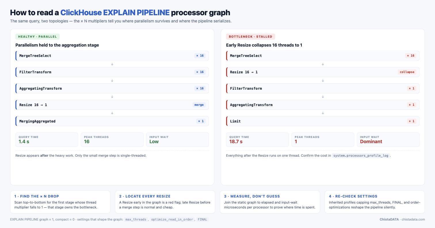
The Three EXPLAIN Levels — and Why PIPELINE Is the One That Finds Stalls
ClickHouse exposes several EXPLAIN modes (all since 20.6): EXPLAIN AST, EXPLAIN SYNTAX, EXPLAIN PLAN (the default), and EXPLAIN PIPELINE. The first three describe what the server intends logically (see the official EXPLAIN reference for the complete modifier list). Only PIPELINE describes the physical processor graph — the units of work the executor actually schedules onto threads. A query execution plan can look perfectly reasonable while its pipeline serializes 90% of the work through one processor; you will never see that from EXPLAIN PLAN alone.
EXPLAIN PIPELINE
SELECT
    user_id,
    count() AS events
FROM events_local
WHERE event_date >= today() - 7
GROUP BY user_id
ORDER BY events DESC
LIMIT 100;
Typical output shape (annotations added):
(Expression)
ExpressionTransform × 1                 -- final projection: single thread, fine (tiny data)
  (Limit)
  Limit
    (Sorting)
    MergingSortedTransform 16 → 1       -- 16 sorted streams merge into one: expected narrow point
      MergeSortingTransform × 16
        PartialSortingTransform × 16
          (Aggregating)
          Resize 16 → 16
            AggregatingTransform × 16   -- parallel pre-aggregation: this is where the work should be
              (Expression)
              ExpressionTransform × 16
                (ReadFromMergeTree)
                MergeTreeSelect(pool: ReadPool, algorithm: Thread) × 16
Reading a ClickHouse EXPLAIN PIPELINE Graph: Four Checks First
1. Thread multipliers (× N)
The × N suffix is the parallelism of that stage, bounded by max_threads. Read the graph bottom-up (data flows from sources at the bottom to the result at the top) and watch where N drops. A drop is not automatically bad — final merges are inherently narrow — but a drop early in the graph, before the heavy stage, is a parallelism collapse worth fixing.
2. Resize processors
Resize A → B redistributes streams across thread counts. Resize 1 → 16 after a source means ClickHouse produced data single-threaded and is fanning it out afterwards — the expensive part already happened on one core. Common causes: a table function or external source that reads serially, FINAL on older versions, or a single huge unsplittable part.
3. Aggregation topology
Healthy parallel aggregation shows AggregatingTransform × N followed by a merge stage. If instead you see the merge phase dominating wall-clock (confirm with system.query_log ProfileEvents, e.g. AggregationPreallocatedElementsInHashTables and elapsed breakdown from system.processors_profile_log, available since ClickHouse 22.x with log_processors_profiles = 1), the culprit is usually very high cardinality keys forcing a massive two-level hash-table merge on few threads.
4. Sorting topology
PartialSortingTransform × N → MergeSortingTransform × N → MergingSortedTransform N → 1 is the standard pattern. If MergeSortingTransform spills (check ProfileEvents['ExternalSortWritePart'] in query_log), the sort exceeded max_bytes_before_external_sort and went to disk — the pipeline shape is fine but each stage got slower by an order of magnitude.
Production Pattern Catalog: Pipeline Shapes That Signal Trouble
| Pipeline signature | Meaning | Primary fix direction |
|---|---|---|
MergeTreeSelect ... × 1 on a large table | Read parallelism collapsed — often one giant part, or max_threads = 1 inherited from a profile | Check system.parts part sizes; verify max_threads in system.settings |
Resize 16 → 1 before AggregatingTransform × 1 | Serialized aggregation, e.g. some GROUP BY + LIMIT BY / window shapes | Restructure query; pre-aggregate in a subquery; check optimize_aggregation_in_order side effects |
Long chain of ExpressionTransform stages | Per-row function overhead (JSON extraction, regex) dominating | Confirm CPU hotspot in system.trace_log; materialize computed columns |
CreatingSetsTransform feeding a JoiningTransform × 1 | Right-side hash table build for a JOIN — build phase is single-threaded on older versions; parallel hash join since ClickHouse 24.x defaults | Reduce right-table size; set join_algorithm = 'parallel_hash' (available since 22.x) |
From Static Graph to Measured Stalls: processors_profile_log
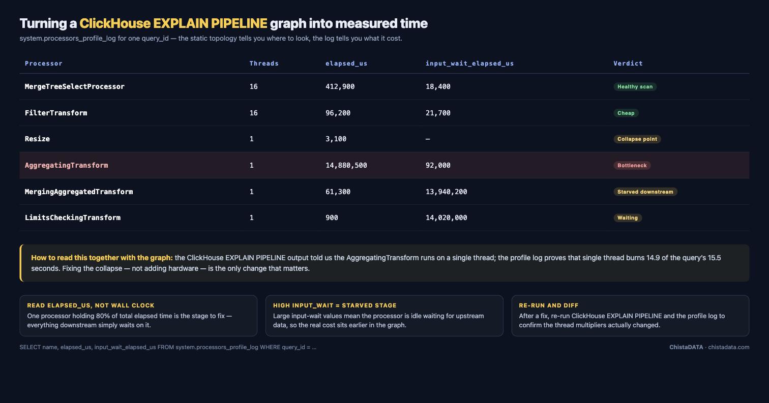
ClickHouse EXPLAIN PIPELINE shows structure; it does not show time. To attribute wall-clock to processors, enable per-processor profiling for the session and read system.processors_profile_log (since ClickHouse 22.x):
Each pattern below is described the way it actually appears in ClickHouse EXPLAIN PIPELINE output, so you can match the shape on screen first and reach for a fix second.
SET log_processors_profiles = 1;

-- run the target query, then:
SELECT
    name,
    count()                                   AS instances,
    sum(elapsed_us)      / 1e6                AS busy_s,
    sum(input_wait_elapsed_us)  / 1e6         AS waiting_for_input_s,
    sum(output_wait_elapsed_us) / 1e6         AS blocked_on_output_s
FROM system.processors_profile_log
WHERE query_id = ${TARGET_QUERY_ID}
GROUP BY name
ORDER BY busy_s DESC;
The three time columns are the stall diagnosis: high input_wait means the stage upstream is the bottleneck (this stage is starved); high output_wait means the stage downstream cannot absorb output (backpressure); high elapsed means this stage itself is the hot one. This turns “the query is slow” into “MergingAggregatedTransform accounts for 71% of busy time and everything above it is starved” — an actionable statement.
Distributed Queries: What ClickHouse EXPLAIN PIPELINE Does and Doesn’t Show
Run against a Distributed table, ClickHouse EXPLAIN PIPELINE on the initiator shows the local plan plus remote-source processors (Remote / ReadFromRemote) — it does not expand the pipeline that will execute on each shard. The initiator’s graph answers one question well: what happens to shard results after they arrive. A MergingAggregatedTransform or sorting merge with a low × N above the remote sources tells you the coordinator is the convergence bottleneck, which pairs with the classic symptom of the initiator node running hot while shards idle.
In other words, ClickHouse EXPLAIN PIPELINE is per-node: to understand a distributed bottleneck you have to collect the graph from the initiator and from at least one shard replica.
To see the shard-side pipeline, run the same EXPLAIN directly against the local table on a shard (or via clusterAllReplicas for telemetry tables). Two settings change the distributed pipeline’s shape and are worth verifying in system.settings when graphs don’t match expectations: distributed_aggregation_memory_efficient (streams partial aggregates so the initiator merges incrementally) and optimize_distributed_group_by_sharding_key (lets sharding-key-aligned GROUP BYs complete on shards entirely, collapsing the coordinator’s merge stage to a concatenation).
Readable Output at Scale: compact and graph Modifiers
Real production pipelines run to hundreds of processors, and the default text tree becomes hard to diff or archive. Two modifiers help:
On wide production queries, run ClickHouse EXPLAIN PIPELINE with the compact modifier first for a quick shape check, then switch to the graph form when you need the exact processor wiring.
-- Collapse repeated processors into the × N notation (default is 1 in modern builds):
EXPLAIN PIPELINE compact = 1
SELECT ...;

-- Emit DOT format for Graphviz rendering - ideal for change reviews:
EXPLAIN PIPELINE graph = 1
SELECT ...
FORMAT TSVRaw;
-- pipe through: dot -Tsvg > pipeline.svg
The Graphviz output earns its keep in change management: attach the before/after SVG of a pipeline to the review for an index, projection, or settings change, and the parallelism impact is visible to reviewers who never read the SQL. We keep rendered pipelines alongside p99 baselines in customer runbooks for exactly this reason — a shape regression after an upgrade is caught by diffing two images, not by re-deriving expectations from memory. One caution: processor names and graph layout evolve between ClickHouse releases (names visible in 23.x differ in places from 21.x), so archive the server version string with every saved pipeline and re-baseline after upgrades rather than diffing across versions.
Worked Example: The Single-Threaded FINAL
A recurring engagement pattern (anonymized): a ReplacingMergeTree-backed API query using FINAL was fast on a fresh table and degraded weekly. ClickHouse EXPLAIN PIPELINE showed the select stage collapsing toward few effective streams as the part count per partition grew, with deduplicating merge stages narrowing the graph. The measured confirmation came from part counts in system.parts and the pipeline’s merge fan-in; the fix was operational, not query-level: tighter partitioning, scheduled OPTIMIZE during low-traffic windows on the affected partitions (gated by an explicit change-approval step, with part-count verification queries before and after), and on ClickHouse 23.x+, do_not_merge_across_partitions_select_final = 1 to let FINAL parallelize across partitions. Pipeline shape before/after made the improvement reviewable by people who never read the query.
The Settings That Shape Every Pipeline
Before attributing a pipeline shape to the query, verify the settings that determine it, because inherited profiles are a chronic source of mystery serialization. max_threads caps the × N multipliers and defaults to physical core count, but a BI tool’s connection profile pinning it to 4 will make every pipeline from that tool look “collapsed.” max_streams_to_max_threads_ratio lets the reader open more streams than threads to smooth uneven part sizes.
optimize_read_in_order and optimize_aggregation_in_order trade parallel scan shapes for order-exploiting shapes — often a win for LIMIT queries aligned with the sort key, but they change the graph substantially and can reduce parallelism on unaligned workloads, so a shape diff after enabling them is expected, not alarming. Check the effective values for the exact session that produced a suspicious graph:
SELECT
    name,
    value,
    changed
FROM system.settings
WHERE name IN
(
    'max_threads',
    'max_streams_to_max_threads_ratio',
    'optimize_read_in_order',
    'optimize_aggregation_in_order',
    'join_algorithm'
)
ORDER BY name;
As always: reproduce the pipeline in a staging environment on production-shaped data before applying settings or schema changes to production, keep every change reversible, and maintain a robust backup/DR posture — pipeline tuning is safe precisely because it is observational, but the fixes it motivates are not.
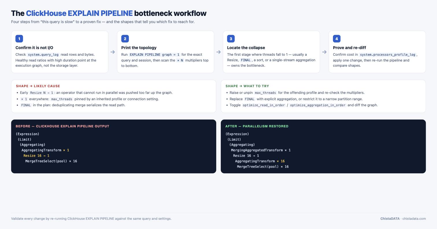
Key Takeaways
- ClickHouse EXPLAIN PIPELINE (since 20.6) shows the physical processor graph — the only EXPLAIN mode that exposes thread counts and serialization points.
- Read bottom-up and track the
× Nmultipliers; an early parallelism collapse matters far more than a narrow final merge. Resize A → Bprocessors mark stream redistribution —Resize 1 → Nafter a source means the expensive read already ran single-threaded.- Structure comes from ClickHouse EXPLAIN PIPELINE; time comes from
system.processors_profile_log(22.x+) — useinput_wait/output_wait/elapsedto separate starved, backpressured, and hot stages. - Common production culprits: single-threaded JOIN build phases, high-cardinality aggregation merges, external sort spills, and
FINALon part-heavy partitions. - Validate every fix by re-running ClickHouse EXPLAIN PIPELINE and comparing p99 in
system.query_log— shape change without latency change means you fixed the wrong stage. - Make a ClickHouse EXPLAIN PIPELINE diff part of the review checklist for every new dashboard query, not just an incident tool.
FAQ
What does ClickHouse EXPLAIN PIPELINE show?
ClickHouse EXPLAIN PIPELINE prints the physical execution graph: the processors (source readers, transforms, merges), how streams connect them, and how many threads (× N) each stage runs on. It is the physical counterpart to the logical EXPLAIN PLAN.
How do I find which stage of a ClickHouse query is slow?
Combine EXPLAIN PIPELINE for structure with system.processors_profile_log (set log_processors_profiles = 1, since 22.x) for per-processor elapsed and wait times, grouped by processor name for the target query_id.
Why is my ClickHouse query only using one thread?
Check max_threads in effect (system.settings), whether the table has one dominant part (system.parts), and whether the query shape forces serialization — e.g. certain FINAL, JOIN build, or ordered-aggregation paths. ClickHouse EXPLAIN PIPELINE shows exactly which stage carries × 1.
What is a Resize processor in a ClickHouse pipeline?
A processor that changes the number of parallel streams between stages (Resize 16 → 8). It exists to rebalance work; its position tells you where parallelism was gained or lost in the plan.
If pipeline analysis keeps pointing at fixes you don’t have bandwidth to engineer, ChistaDATA’s ClickHouse Performance Consulting and 24x7x365 Support (15-minute S1 response SLA) does this work on production clusters every week — on 100% open-source ClickHouse with zero vendor lock-in. Engage a ChistaDATA ClickHouse engineer.
How often should I run ClickHouse EXPLAIN PIPELINE?
Run ClickHouse EXPLAIN PIPELINE whenever a query shape changes: after a schema or sort key change, after a settings profile update, and before promoting a new dashboard query to production. The graph is cheap to print because nothing is executed, so treating it as a pre-flight check costs nothing and catches serialization before users do.
Running ClickHouse in production? ChistaDATA provides ClickHouse consulting for architecture, performance and migrations, and 24×7 ClickHouse support with a 15-minute S1 response. For day-to-day operations see ClickHouse DBA services and ClickHouse managed services.
