“The dashboards feel slower this week” is not an incident report — it is a hypothesis. Turning it into an engineering decision requires disciplined ClickHouse latency analysis: a baseline, a regression-detection query, and an attribution step, all built on system.query_log. This playbook documents the Data SRE workflow ChistaDATA runs for customers with latency SLOs on ClickHouse: how to baseline p95/p99 per query shape, how to detect regressions statistically rather than anecdotally, and how to attribute a regression to code, data, or environment before anyone touches a setting. It assumes production ClickHouse and an audience already fluent in MergeTree operations.
ClickHouse Latency Analysis Basics: Why p95/p99, and Why per Query Shape
Proper ClickHouse latency analysis treats SLOs as commitments about the experience of nearly all requests, so the tail is the contract: p50 can improve while p99 doubles, and users will correctly report a regression. Equally important, cluster-wide percentiles are almost useless — a workload-mix shift (more heavy exports, fewer cheap lookups) moves the global p99 with zero per-query regression. The unit of analysis must be the query shape: normalized_query_hash (since ClickHouse 21.x), which strips literals so all parameterizations of a statement aggregate together.
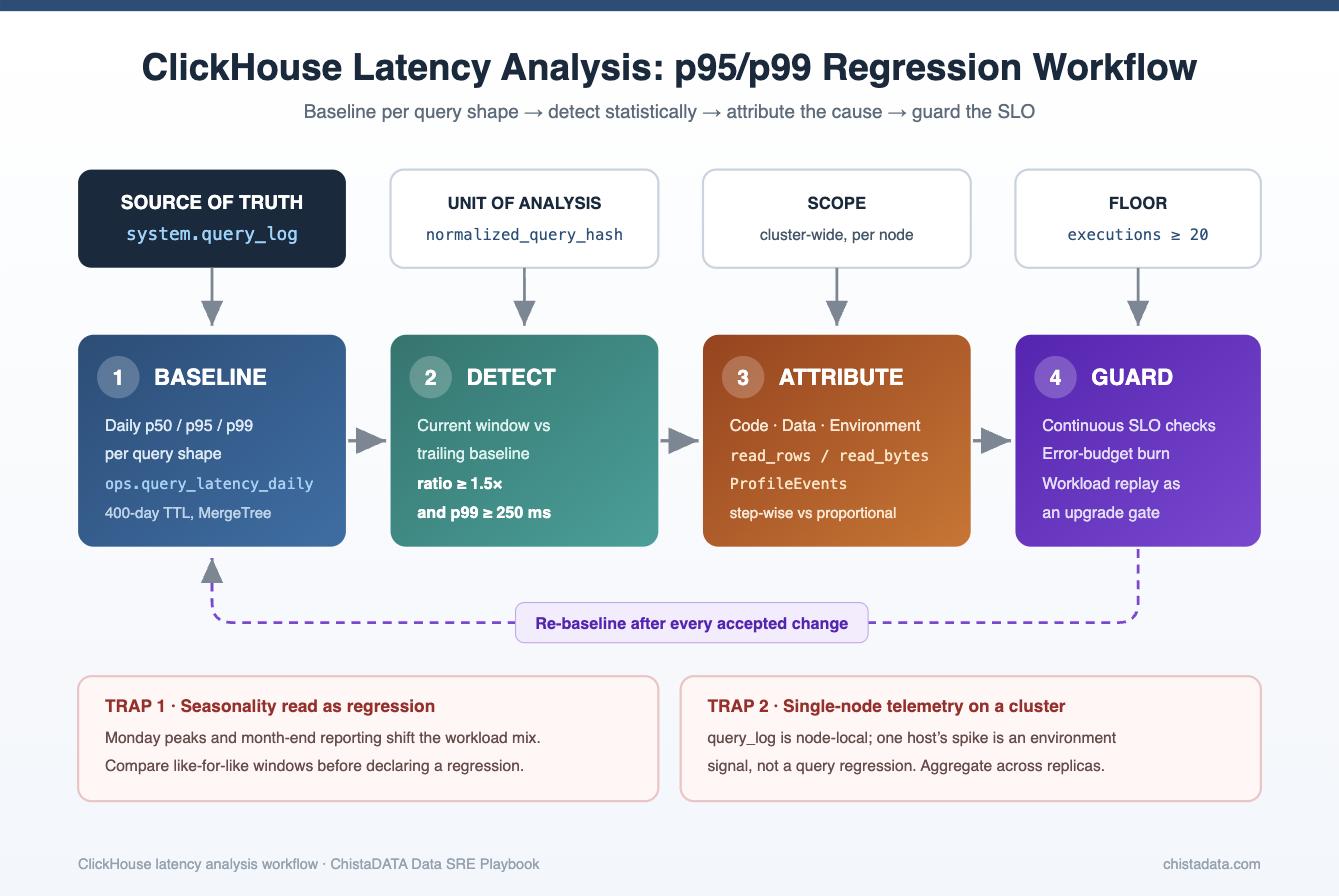
system.query_log: baseline per query shape, detect statistically, attribute the cause, then guard the SLO.Step 1 — Build the ClickHouse Latency Analysis Baseline Table
Durable ClickHouse latency analysis starts by persisting daily latency profiles per query shape instead of recomputing them ad hoc (the query_log column reference documents every field used below). A small aggregating pipeline over query_log is enough — explicit engine, no defaults:
CREATE TABLE ops.query_latency_daily
(
    day                    Date,
    normalized_query_hash  UInt64,
    sample_query           String,
    executions             UInt64,
    p50_ms                 Float64,
    p95_ms                 Float64,
    p99_ms                 Float64,
    read_rows_p95          Float64,
    memory_p95             Float64
)
ENGINE = ReplicatedMergeTree('/clickhouse/tables/{shard}/ops/query_latency_daily', '{replica}')
PARTITION BY toYYYYMM(day)
ORDER BY (normalized_query_hash, day)
TTL day + INTERVAL 400 DAY DELETE
SETTINGS index_granularity = 8192;

INSERT INTO ops.query_latency_daily
SELECT
    today() - 1                                        AS day,
    normalized_query_hash,
    any(query)                                         AS sample_query,
    count()                                            AS executions,
    quantile(0.50)(query_duration_ms)                  AS p50_ms,
    quantile(0.95)(query_duration_ms)                  AS p95_ms,
    quantile(0.99)(query_duration_ms)                  AS p99_ms,
    quantile(0.95)(read_rows)                          AS read_rows_p95,
    quantile(0.95)(memory_usage)                       AS memory_p95
FROM system.query_log
WHERE type = 'QueryFinish'
  AND is_initial_query = 1
  AND event_date = today() - 1
GROUP BY normalized_query_hash
HAVING executions >= 20;
The HAVING executions >= 20 floor matters: a p99 computed from six executions is noise, and alerting on it will train your team to ignore the alert. Schedule the INSERT daily (cron, Airflow, or a refreshable materialized view on ClickHouse 24.x+ — the latter should be validated in staging first, as refreshable MVs are a newer feature).
Step 2 — The Regression Detection Query
ClickHouse latency analysis becomes operational at this step: compare a current window against a trailing baseline and rank by regression ratio, filtering for both statistical floor and absolute materiality:
WITH
    baseline AS
    (
        SELECT
            normalized_query_hash,
            quantile(0.99)(p99_ms) AS p99_baseline,
            sum(executions)        AS exec_baseline
        FROM ops.query_latency_daily
        WHERE day BETWEEN today() - 28 AND today() - 8
        GROUP BY normalized_query_hash
    ),
    current AS
    (
        SELECT
            normalized_query_hash,
            any(sample_query)      AS sample_query,
            quantile(0.99)(p99_ms) AS p99_current,
            sum(executions)        AS exec_current
        FROM ops.query_latency_daily
        WHERE day >= today() - 7
        GROUP BY normalized_query_hash
    )
SELECT
    c.sample_query,
    b.p99_baseline,
    c.p99_current,
    round(c.p99_current / b.p99_baseline, 2) AS regression_ratio,
    c.exec_current
FROM current AS c
INNER JOIN baseline AS b
    ON c.normalized_query_hash = b.normalized_query_hash
WHERE c.p99_current > b.p99_baseline * 1.5
  AND c.p99_current > 250            -- ignore sub-250ms noise; tune to your SLO
  AND c.exec_current >= 100
ORDER BY regression_ratio DESC
LIMIT 25;
The 1.5× threshold, 250 ms floor, and window sizes are policy, not physics — set them from your SLO and error budget. Teams running formal SLOs typically wire this query into their burn-rate alerting: a shape regressing 3× that consumes meaningful error budget pages someone; a 1.6× regression on a nightly batch query files a ticket.
Step 3 — Attribute Before You Tune
Attribution is the step teams skip most often. Every query performance regression that ClickHouse latency analysis surfaces has one of four causes. The query_log columns for the regressed shape, compared across the baseline and current windows, discriminate between them:
| Cause | Discriminating signal (baseline → current) | Confirm with |
|---|---|---|
| Data growth / distribution shift | read_rows, read_bytes grew proportionally with latency | system.parts rows/bytes trend for target tables |
| Plan/index change | read_rows jumped step-wise; ProfileEvents['SelectedMarks'] up sharply | EXPLAIN indexes = 1 now vs expected; recent DDL in system.query_log (query_kind = 'Create'/'Alter') |
| Environment / contention | Read metrics flat, latency up; OSCPUWaitMicroseconds up | system.merges backlog, system.mutations with is_done = 0, co-tenant query volume in the same window |
| Server change (version, settings) | Regression aligned to a deploy timestamp across many shapes at once | system.settings diff; server restart events in logs |
The step-wise vs proportional distinction does most of the work. Proportional growth in read_rows is a capacity conversation; a step change with unchanged data volume is a plan conversation; flat reads with rising wall-clock is a contention conversation. Tuning settings before this attribution step is how clusters accumulate cargo-cult configuration. When attribution does point at the plan, ClickHouse MergeTree optimization — sort keys, partitioning, and skip indexes — is usually where the real fix lives.
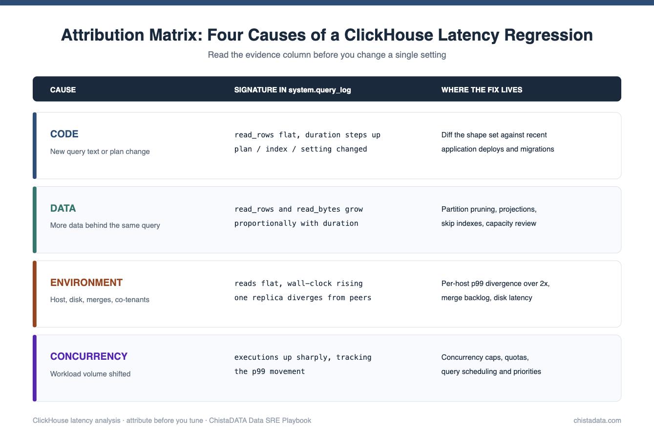
system.query_log.Work the matrix top to bottom rather than guessing. In practice, ClickHouse latency analysis resolves most escalations on the first two rows, and the remainder are usually environmental rather than anything a settings change would repair.
Two Traps That Corrupt ClickHouse Latency Analysis Baselines
Trap 1: Seasonality read as regression
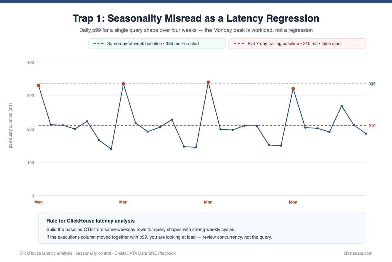
ClickHouse latency analysis has to respect the fact that analytical workloads breathe: Monday-morning dashboard storms, month-end closes, marketing-campaign spikes. A same-day-of-week comparison is the cheap defense — compare this Monday against the trailing four Mondays, not against Sunday. In the detection query, that means building the baseline CTE from toDayOfWeek(day) = toDayOfWeek(today()) rows rather than a flat trailing window for shapes with strong weekly cycles. The executions column doubles as the seasonality signal: if execution volume moved 3× along with p99, you are looking at load, not regression, and the correct response is a concurrency/capacity review rather than query tuning.
Trap 2: Single-node telemetry on a multi-node cluster
ClickHouse latency analysis breaks down quietly here, because system.query_log is node-local. A baseline built from one replica silently excludes every query routed elsewhere by your load balancer, and per-node performance asymmetries (degraded disk, noisy co-tenant VM) vanish into the aggregate. Collect fleet-wide and keep the host dimension:
SELECT
    hostName()                                         AS host,
    normalized_query_hash,
    count()                                            AS executions,
    quantile(0.99)(query_duration_ms)                  AS p99_ms
FROM clusterAllReplicas(${CLUSTER_NAME}, system.query_log)
WHERE type = 'QueryFinish'
  AND is_initial_query = 1
  AND event_date = today() - 1
GROUP BY host, normalized_query_hash
HAVING executions >= 20
ORDER BY p99_ms DESC;
Retention policy follows from this split: keep the host-level daily aggregates as long as the shape-level ones, because post-hoc infrastructure investigations (“when did replica 3 start diverging?”) need exactly the history that ad hoc queries against an expired raw log can no longer provide.
A shape that regressed on one host only is an infrastructure ticket (check that host’s system.parts layout, disk latency, and merge backlog), not a query ticket. Fold the host column into ops.query_latency_daily and alert on per-host divergence — replicas whose p99 for the same shape differs by more than ~2× — separately from shape-level regression. In our experience this single split resolves a large fraction of “the query got slower” escalations without touching a line of SQL, because the query never changed; a replica did.
Step 4 — Guard the SLO Continuously, Not Forensically
Once baselining and detection run daily, two additions turn ClickHouse latency analysis into a real SRE control loop rather than a post-incident tool. Both assume a working ClickHouse performance observability and monitoring foundation underneath:
- Release gates — run the regression query with a 24-hour window after each application deploy or ClickHouse upgrade; a new step-change regression blocks promotion. ClickHouse upgrades in particular should always pass this gate in staging with production-shaped workload replay first.
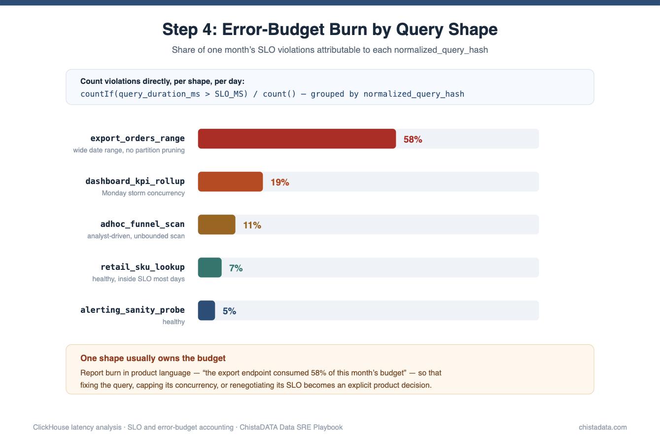
- Error-budget accounting — count SLO-violating executions directly:
countIf(query_duration_ms > ${SLO_MS})overquery_logper day, per shape. Budget burn per shape identifies which single query shape is spending your reliability budget — frequently one shape accounts for the majority of violations (verify on your own data; this ratio varies widely by workload). Report burn in user-meaningful units: “the export endpoint consumed 60% of this month’s budget” lands with product owners in a way that milliseconds never will, and it makes the prioritization conversation — fix the query, cap its concurrency, or renegotiate its SLO — an explicit product decision rather than an engineering default.
Closing the loop with workload replay
Deploy gates are only as honest as the workload they test against, and synthetic benchmarks systematically miss the query shapes that actually regress. The pragmatic answer is replay from query_log itself: export the distinct QueryFinish statements for your top-N shapes over a representative window, weight them by observed execution counts, and run them against the staging candidate (new ClickHouse version, new schema, new settings profile) with clickhouse-benchmark or a simple driver.
Two disciplines make the comparison valid: replay against a data snapshot restored from the same backup lineage as production — which conveniently doubles as a periodic restore test for your DR posture — and pin max_threads and memory settings identically on both sides so you are measuring the change, not the environment.
Record the replay’s per-shape p95/p99 into the same ops.query_latency_daily schema with a distinguishing environment column, and the regression query from Step 2 becomes your upgrade gate with zero new tooling.
All figures and thresholds in this post are illustrative policy defaults, not benchmarks. And the standing rule applies to every remediation this playbook triggers: test in staging before production, prefer staged and reversible changes, and maintain a robust backup and DR posture — latency work must never compromise durability.
Key Takeaways for ClickHouse Latency Analysis
- SLO-grade ClickHouse latency analysis is per query shape (
normalized_query_hash), never cluster-wide — workload mix shifts corrupt global percentiles. - Persist daily p50/p95/p99 profiles from
system.query_loginto an explicit ReplicatedMergeTree baseline table with a TTL. - Detect regressions with a windowed comparison (current vs trailing baseline) gated by ratio, absolute latency, and execution-count floors.
- Attribute before tuning: proportional
read_rowsgrowth = data; step change = plan; flat reads with rising latency = contention; fleet-wide shift at a timestamp = server change. - Continuous ClickHouse latency analysis means wiring the detection query into deploy gates and error-budget burn accounting to move from forensic to continuous control.
- Thresholds are policy — derive them from your SLO, and validate every fix against the same baseline that caught the regression.
ClickHouse Latency Analysis FAQ
How do I measure p99 latency in ClickHouse?
Use quantile(0.99)(query_duration_ms) over system.query_log filtered to type = 'QueryFinish' and is_initial_query = 1, grouped by normalized_query_hash so each query shape gets its own percentile.
Why did my ClickHouse query suddenly get slower?
Compare read_rows, read_bytes, and ProfileEvents for the shape across before/after windows. Proportional read growth points to data volume; a step change points to a plan or index regression; unchanged reads with higher latency point to contention from merges, mutations, or co-tenant load.
What is a good latency SLO for ClickHouse?
There is no universal number — it depends on workload class. The defensible ClickHouse latency analysis method is to baseline current p95/p99 per critical query shape, set the SLO slightly above the healthy baseline, and manage it with error budgets rather than picking a round number.
How long should I keep system.query_log data?
Keep the raw log weeks (TTL on the log engine) and persist compact daily aggregates for a year or more in your own baseline table. Regression detection needs long history; the raw log does not have to provide it.
How often should ClickHouse latency analysis run?
Daily is the right default for baselining and detection: it is cheap against pre-aggregated rows and it keeps the trailing window honest. Run the detection query on demand as well after every deploy, schema migration, and version upgrade, because those are the moments when a step-change regression is most likely and cheapest to reverse.
ChistaDATA operates exactly this ClickHouse latency analysis playbook — baselining, regression alerting, attribution, and remediation — as part of ClickHouse Performance Consulting and 24x7x365 Support with a 15-minute S1 SLA, on 100% open-source ClickHouse with zero vendor lock-in. If you’d rather inherit a working SLO practice than build one mid-incident, talk to ChistaDATA.
Running ClickHouse in production? ChistaDATA provides ClickHouse consulting for architecture, performance and migrations, and 24×7 ClickHouse support with a 15-minute S1 response. For day-to-day operations see ClickHouse DBA services and ClickHouse managed services.
