The ClickHouse query profiler is a sampling profiler built into the server: switch it on for a session, run the query, and system.trace_log fills with stack samples that say where the wall-clock and CPU time went, function by function. It answers the question the query log cannot, which is not “how long did this take” but “in which part of the engine, doing what”.
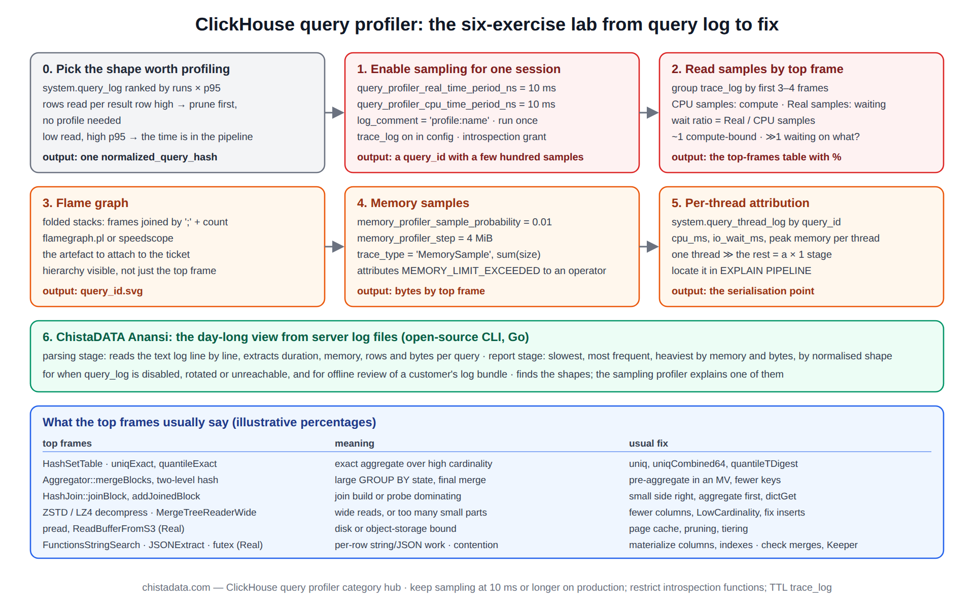
This page is written as a lab: a sequence of exercises that take a slow query from the log to a flame graph and back to a fix, each with the exact settings, the query that reads the samples, and what the output looks like. It closes with the log-based profiler ChistaDATA built, Anansi, which does for a day of query logs what the sampling profiler does for one statement.
The posts in this category cover the tools around the profiler: EXPLAIN PIPELINE, query_thread_log, thread contention, the essential metrics, the configuration variables, and the two posts introducing Anansi. The lab below is the sequence they fit into.
Exercise 0: choose a query worth the ClickHouse query profiler’s time
Profiling is cheap per query and expensive per engineer-hour, so the first exercise is picking the right statement. The query log ranks shapes by total time (runs multiplied by p95), and the shape at the top of that ranking is the one to profile, not the single slowest query, which is often a one-off export.
Two columns decide whether profiling will help at all: if read_rows per result row is enormous, the problem is pruning and EXPLAIN indexes = 1 answers it without a profile; if read volume is modest and the query is still slow, the time is inside the pipeline and the profiler is the right tool.
SELECT
    normalized_query_hash                                  AS shape,
    count()                                                AS runs,
    quantile(0.95)(query_duration_ms)                      AS p95_ms,
    round(count() * quantile(0.95)(query_duration_ms) / 1000) AS weighted_s,
    round(avg(read_rows) / greatest(avg(result_rows), 1))  AS rows_per_result,
    any(substring(query, 1, 100))                          AS sample
FROM system.query_log
WHERE type = 'QueryFinish' AND query_kind = 'Select'
  AND event_time > now() - INTERVAL 7 DAY
GROUP BY shape
ORDER BY weighted_s DESC
LIMIT 10;
-- rows_per_result in the thousands → pruning first; low rows_per_result and high p95 → profile it
Exercise 1: turn the ClickHouse query profiler on for one query
Two settings control sampling. query_profiler_real_time_period_ns samples on wall-clock time and catches waiting (I/O, locks, network); query_profiler_cpu_time_period_ns samples on CPU time and catches compute. Both default to 1 second in older releases and to 10 ms of CPU sampling in recent ones for queries that run long enough; for a deliberate profile, 10 ms (10,000,000 ns) on both is safe on production and gives a few hundred samples for a multi-second query. Set them in the session, tag the query so it can be found, and run it once.
SET query_profiler_real_time_period_ns = 10000000;   -- 10 ms wall clock
SET query_profiler_cpu_time_period_ns  = 10000000;   -- 10 ms CPU
SET log_comment = 'profile:slow-dashboard-1';

SELECT tenant_id, uniqExact(user_id), sum(amount_cents)
FROM events
WHERE event_date >= today() - 30
GROUP BY tenant_id;

-- find its query_id afterwards
SELECT query_id, query_duration_ms, read_rows, memory_usage
FROM system.query_log
WHERE log_comment = 'profile:slow-dashboard-1' AND type = 'QueryFinish'
ORDER BY event_time DESC LIMIT 1;
trace_log must be enabled in the server config (<trace_log> section, on by default in packaged configs) and the symbol-resolving functions need allow_introspection_functions = 1, which is a per-user grant worth restricting to the engineers who profile.
Exercise 2: read the samples by top frame
The raw table has one row per sample with a trace array of addresses. Grouping by the top few frames and counting samples gives the profile; trace_type separates CPU from Real samples so that the two questions (compute vs waiting) are answered separately. The query below is the one to save; it is the ClickHouse query profiler’s equivalent of a perf report.
SET allow_introspection_functions = 1;

SELECT
    trace_type,
    count()                                                              AS samples,
    round(count() * 100.0 / sum(count()) OVER (PARTITION BY trace_type), 1) AS pct,
    arrayStringConcat(
        arrayMap(x -> demangle(addressToSymbol(x)), arraySlice(trace, 1, 4)), ' ← ') AS top_frames
FROM system.trace_log
WHERE query_id = '${QUERY_ID}'
  AND trace_type IN ('CPU', 'Real')
GROUP BY trace_type, top_frames
ORDER BY trace_type, samples DESC
LIMIT 10 BY trace_type;

-- illustrative output for the uniqExact query
-- CPU   61%  HashSetTable::emplace ← AggregateFunctionUniqExact::add ← Aggregator::executeImpl ← AggregatingTransform::work
-- CPU   18%  ZSTD_decompressBlock ← CompressedReadBuffer::nextImpl ← MergeTreeReaderWide::readRows
-- Real  44%  pread ← ReadBufferFromFileDescriptor::readImpl ← ...   (waiting on disk)
The percentages are the whole point of the table, and they are read against each other rather than in isolation. Reading it: 61 percent of CPU inside the uniqExact hash set means the aggregation function is the cost, and switching to uniq (a sketch) is the fix; the Real profile’s 44 percent in pread says the read is disk-bound for nearly half the wall time, which is a separate finding about the page cache or the columns read.
Exercise 3: build a flame graph from the ClickHouse query profiler output
A table of top frames is enough for a quick decision; a ticket that another engineer will act on deserves the picture. The same samples, exported in folded-stack format, feed Brendan Gregg’s flamegraph.pl or any speedscope-style viewer. Each line is the full stack joined by semicolons and the sample count; the visual makes the hierarchy obvious in a way a top-frames table does not, and it is the format to attach to a ticket.
clickhouse-client --query "
SELECT
    arrayStringConcat(arrayReverse(arrayMap(x -> demangle(addressToSymbol(x)), trace)), ';') AS stack,
    count() AS samples
FROM system.trace_log
WHERE query_id = '${QUERY_ID}' AND trace_type = 'CPU'
GROUP BY stack
FORMAT TabSeparated
SETTINGS allow_introspection_functions = 1
" > /tmp/${QUERY_ID}.folded

flamegraph.pl --title "${QUERY_ID} CPU" /tmp/${QUERY_ID}.folded > /tmp/${QUERY_ID}.svg
Exercise 4: memory samples and the allocation profile
Besides time, the profiler samples allocations. With memory_profiler_sample_probability set (0.01 samples one allocation in a hundred) and memory_profiler_step set, trace_log gains MemorySample and Memory rows whose size column is the allocation size, so the same top-frames query grouped on trace_type = 'MemorySample' with sum(size) instead of count() shows which operator is holding memory. This is how a MEMORY_LIMIT_EXCEEDED is attributed to a hash join build side, a GROUP BY state, or a sort buffer, and the memory hub takes the finding from there.
SET memory_profiler_sample_probability = 0.01;
SET memory_profiler_step = 4194304;     -- 4 MiB: also log a sample every 4 MiB of growth

SELECT
    formatReadableSize(sum(size))                                   AS sampled_bytes,
    arrayStringConcat(arrayMap(x -> demangle(addressToSymbol(x)), arraySlice(trace, 1, 3)), ' ← ') AS top_frames
FROM system.trace_log
WHERE query_id = '${QUERY_ID}' AND trace_type = 'MemorySample'
GROUP BY top_frames
ORDER BY sum(size) DESC
LIMIT 8
SETTINGS allow_introspection_functions = 1;
Exercise 5: per-thread attribution with query_thread_log
The profiler says where time went; system.query_thread_log says which threads did the work and how evenly. A query with max_threads = 16 whose thread log shows one thread with ten times the CPU of the others has a serialisation point, which EXPLAIN PIPELINE then locates as the step with × 1. The query_thread_log post covers the table; the thread contention post covers what to do when the threads are all busy and still slow.
SELECT
    thread_id,
    thread_name,
    round(ProfileEvents['OSCPUVirtualTimeMicroseconds'] / 1000)  AS cpu_ms,
    round(ProfileEvents['OSIOWaitMicroseconds'] / 1000)          AS io_wait_ms,
    formatReadableSize(peak_memory_usage)                          AS peak_mem,
    read_rows
FROM system.query_thread_log
WHERE query_id = '${QUERY_ID}'
ORDER BY cpu_ms DESC;
-- one thread far above the rest = a single-threaded stage; find it in EXPLAIN PIPELINE
Exercise 6: the day-long view with Anansi, ChistaDATA’s log-based ClickHouse query profiler
The sampling profiler explains one query. Anansi explains a day. It is an open-source CLI tool written in Go, built by ChistaDATA, that reads ClickHouse server log files (the text logs, not system tables), extracts every query’s execution time, memory, rows and bytes read with regular expressions in a parsing stage, and produces a report in a generation stage: the slowest queries, the most frequent, the heaviest by memory and by bytes, grouped by normalised shape.
It is the tool for the situation where system.query_log is disabled, rotated, or on a server that cannot be queried, and for the offline review of a log bundle a customer sends with a ticket. The two archive posts, introducing Anansi and the profiler walkthrough, cover installation, supported log formats and the report.
# illustrative invocation; see the Anansi posts for the current flags
anansi --log /var/log/clickhouse-server/clickhouse-server.log \
       --top 20 \
       --sort duration \
       --report /tmp/anansi-report.txt

# the report answers the question-1 table of a performance review from logs alone:
# shape, count, total time, p95, avg rows read, avg memory
The two profilers are complementary, and a ClickHouse query profiler session normally uses both. Anansi (or a system.query_log query when the table is available) finds the shapes worth profiling; the sampling profiler explains why one of them is slow; the fix is validated by running the shape again under both.
Reading the gap between Real and CPU samples in ClickHouse query profiler output
The two sample streams are most useful together. A query whose CPU samples and Real samples land in the same frames is compute-bound and the fix is in the query or the schema. A query whose Real samples sit in pread, ReadBufferFromS3 or a socket read while its CPU samples are few is waiting, and the fix is in storage, the page cache or the network.
A query whose Real samples sit in futex or a condition-variable wait is contended, usually with merges, a mutation, or Keeper, and the fix is elsewhere on the node entirely. The ratio of Real to CPU sample counts for the same query is itself a number worth recording: near 1 means the query is running, well above 1 means it is waiting, and the profile says on what.
SELECT
    countIf(trace_type = 'Real') AS real_samples,
    countIf(trace_type = 'CPU')  AS cpu_samples,
    round(real_samples / greatest(cpu_samples, 1), 2) AS wait_ratio
FROM system.trace_log
WHERE query_id = '${QUERY_ID}';
-- wait_ratio ~1: compute-bound · >>1: waiting; read the Real top frames to see on what
Profiling merges and background work with the ClickHouse query profiler
The profiler is not only for queries. Background merges, mutations and fetches run on server threads and appear in system.trace_log with a query_id that identifies the merge (visible in system.merges and in system.part_log), so a merge that takes an hour can be profiled the same way as a query: its top frames show whether the time is in decompression, in the merge algorithm (a ReplacingMergeTree or AggregatingMergeTree collapsing step), in the codec on the write side, or in disk writes.
The global sampling settings apply here rather than session settings, because there is no session; a server-level query_profiler_cpu_time_period_ns of 100 ms is a reasonable standing value that keeps merge profiles available without much overhead. The merge queues post covers where to find the merge to profile.
A worked example, end to end (illustrative)
A dashboard shape at the top of the exercise-0 ranking ran 1,400 times a day at a p95 of 6.8 s. EXPLAIN indexes = 1 showed pruning was fine: 2 percent of granules kept. The CPU profile put 58 percent of samples in uniqExact‘s hash set and 21 percent in ZSTD decompression of a wide String column that the query did not use in its output but named in SELECT *. The Real profile’s wait ratio was 1.1, so the query was compute-bound.
Two changes followed: uniqExact became uniqCombined64 after the product owner confirmed 0.5 percent error was acceptable for the dashboard, and the column list replaced SELECT *.
Re-profiled, the same shape ran at a p95 of 0.7 s with the top frame now in the aggregation merge at 34 percent, which is where a healthy GROUP BY profile sits. The numbers are illustrative of the pattern, not a benchmark; the pattern itself recurs in most engagements.
What the ClickHouse query profiler finds most often
| Top frames | Meaning | Usual fix |
|---|---|---|
| HashSetTable / uniqExact, quantileExact | exact aggregate over high cardinality | uniq, uniqCombined64, quantileTDigest |
| Aggregator::mergeBlocks, two-level hash | large GROUP BY state, final merge | pre-aggregate in an MV; group on fewer keys |
| HashJoin::joinBlock, addJoinedBlock | hash join build or probe dominating | small side right; aggregate first; dictGet |
| ZSTD_decompress, LZ4_decompress | decompression of wide reads | fewer columns; LowCardinality; check codec level |
| pread, ReadBufferFromFileDescriptor (Real) | disk-bound read | page cache, column pruning, sort key, tiering |
| FunctionsStringSearch, ILIKE, match | string scan per row | materialize lower(), tokenbf index, text index |
| JSONExtract*, simdjson | JSON parsed per row | materialize the extracted column; JSON type |
| MergeTreeReaderWide::readRows (many parts) | too many small parts | fix inserts; OPTIMIZE FINAL once, then batching |
| Sort, MergeSortingTransform | ORDER BY over a large set | LIMIT with ORDER BY; sort key alignment; external sort |
| futex, lock wait (Real) | contention, often on Keeper or a mutation | see thread contention post; check merges |
Running the ClickHouse query profiler safely in production
Sampling costs a signal handler per period per thread, so a 10 ms period on a 32-thread query is 3,200 samples per second, which is negligible; a 1 ms period on a hundred concurrent queries is not, and the trace_log table grows fast. Three rules keep it safe. Enable the profiler per session for a named query, not globally in the profile, unless the period is 1 s or longer.
Keep allow_introspection_functions restricted to a profiling role, because addressToSymbol and addressToLine expose binary internals. And set a TTL on system.trace_log (<ttl>event_date + INTERVAL 7 DAY</ttl> in the config’s <trace_log> section) so that a week of samples is the ceiling. The configuration variables post lists the related server settings.
Version notes
The sampling profiler and system.trace_log have been stable since 20.x. The memory profiler settings are 20.x and later. query_thread_log is 20.x and later. Default CPU sampling for long queries changed in 24.x; confirm the effective defaults with SELECT name, value, changed FROM system.settings WHERE name LIKE 'query_profiler%'. Anansi’s flags and supported log formats are documented in its repository and the archive posts, and change with releases. The sampling query profiler documentation is the reference for the settings and functions used above.
Reading the archive
The archive pairs each exercise with a post, and the posts are worth reading in lab order the first time and by symptom afterwards. A ClickHouse query profiler session that follows the six exercises in sequence takes under an hour on a shape from the query log and ends with a flame graph, a memory attribution and a per-thread table, which together are the evidence a fix is proposed against.
Start with the query profiling post for exercises 1 to 3, the query_thread_log post for exercise 5, the two Anansi posts for exercise 6, and the EXPLAIN PIPELINE post for locating what the profile found. The essential-metrics and configuration-variables posts are the surrounding telemetry.
ChistaDATA runs this lab on the customer’s top query shapes at the start of every ClickHouse consulting performance engagement and attaches the flame graphs to the findings, and 24×7 support uses the same sequence on S2 latency tickets. Profile on a replica that is not serving the critical path first, keep sampling periods at 10 ms or longer on production, and validate every fix by re-profiling the same shape.