ClickHouse SQL engineering is the discipline of writing queries that let the engine skip work, because ClickHouse is fast at scanning and decompressing columns and slow at everything it cannot vectorise: hash joins on large right-hand sides, sorts on unsorted input, functions applied to a wide column before a filter, and anything that forces a full scan when the primary key could have pruned it.
This page is ten ClickHouse SQL engineering rewrite rules, each shown as the query we were handed, the query we returned, and the EXPLAIN or system.query_log evidence that separates them. The examples use one events table with the sort key (tenant_id, event_type, event_time).
The posts in this category go further on individual rules: the optimizer, hash GROUP BY and ORDER BY, row counts in execution plans, long-integer queries, overlapping date ranges, indexing and LowCardinality. This page is the checklist to run before any of them.
Rule one of ClickHouse SQL engineering: filter on the sort key first, in sort-key order
The primary index prunes granules only on a prefix of the ORDER BY. A filter on event_time alone, on a table sorted by tenant first, reads every tenant’s granules for that time range; a filter that names the tenant reads a few hundred.
-- Handed to us: reads all tenants for the window
SELECT count()
FROM events
WHERE event_time >= now() - INTERVAL 1 DAY;

-- Returned: leads with the sort-key prefix the query actually has
SELECT count()
FROM events
WHERE tenant_id = 4711
  AND event_time >= now() - INTERVAL 1 DAY;

EXPLAIN indexes = 1 SELECT count() FROM events WHERE tenant_id = 4711 AND event_time >= now() - INTERVAL 1 DAY;
-- PrimaryKey  Parts: 14/62  Granules: 388/51200
When the query genuinely has no tenant, the answer is a projection or a second table sorted by time, not a wider index. The archive post ClickHouse indexing and SQL engineering covers the projection route.
Rule two: never wrap the sort-key column in a function
toDate(event_time) = today() defeats the index because the index holds event_time, not toDate(event_time). ClickHouse can see through a few monotonic functions, but the safe form is a range on the raw column.
-- Handed to us
WHERE toYYYYMM(event_time) = 202609

-- Returned
WHERE event_time >= toDateTime('2026-09-01 00:00:00', 'UTC')
  AND event_time <  toDateTime('2026-10-01 00:00:00', 'UTC')
Rule three: PREWHERE the selective, cheap column explicitly when the optimiser guesses wrong
ClickHouse moves conditions to PREWHERE automatically, but it ranks them by column size, not by selectivity. When a wide payload column carries a highly selective condition and a narrow column carries a loose one, the automatic order reads the wide column for every granule. The archive post Optimal SQL engineering for ClickHouse performance measures the difference.
-- Returned: force the narrow LowCardinality filter first
SELECT tenant_id, count()
FROM events
PREWHERE event_type = 'refund'
WHERE payload LIKE '%chargeback%'
GROUP BY tenant_id;

-- Evidence: read_bytes before and after
SELECT query_duration_ms, read_rows, formatReadableSize(read_bytes) AS read
FROM system.query_log
WHERE type = 'QueryFinish' AND query LIKE '%chargeback%' AND event_date = today()
ORDER BY event_time DESC LIMIT 2;
Rule four: ClickHouse SQL engineering for JOINs, small table right or a dictionary
The default hash join builds the right-hand table in memory. A join with the fact table on the right builds a hash of a billion rows and fails on memory; the same join with the dimension on the right builds a hash of ten thousand. For dimensions that are looked up in many queries, a Dictionary with dictGet removes the join entirely and is evaluated per row without a hash build. The archive’s Complex queries in ClickHouse walks through both.
-- Handed to us: fact table on the right
SELECT c.country, count()
FROM customers AS c
JOIN events AS e ON e.customer_id = c.customer_id
GROUP BY c.country;

-- Returned: dimension on the right, and the dictionary form
SELECT dictGet('customers_dict', 'country', e.customer_id) AS country, count()
FROM events AS e
WHERE e.event_time >= now() - INTERVAL 7 DAY
GROUP BY country;

-- Evidence
EXPLAIN PIPELINE SELECT ... ;   -- look for JoiningTransform vs none, and peak memory in query_log
Rule five: aggregate before you join, not after
In ClickHouse SQL engineering terms, joining a billion events to customers and then grouping moves a billion rows through the join. Grouping events by customer_id first and joining the aggregate moves ten thousand. The rewrite is mechanical and the gain is usually an order of magnitude.
-- Returned
SELECT c.country, sum(agg.events) AS events
FROM
(
    SELECT customer_id, count() AS events
    FROM events
    WHERE event_time >= now() - INTERVAL 7 DAY
    GROUP BY customer_id
) AS agg
JOIN customers AS c ON c.customer_id = agg.customer_id
GROUP BY c.country;
Rule six: use the aggregate combinators instead of subqueries
ClickHouse’s -If, -Array, -Merge and -State combinators, together with argMax, uniq and quantile families, replace most correlated subqueries and self-joins. A query that joins a table to itself to find each key’s latest row is an argMax; one that runs three passes for three conditions is three countIf columns in one pass. The archive post ClickHouse hash GROUP BY and ORDER BY explains why one pass matters.
-- Handed to us: three scans
SELECT
    (SELECT count() FROM events WHERE event_type = 'purchase' AND event_date = today()) AS purchases,
    (SELECT count() FROM events WHERE event_type = 'refund'   AND event_date = today()) AS refunds,
    (SELECT uniq(customer_id) FROM events WHERE event_date = today())                  AS customers;

-- Returned: one scan
SELECT
    countIf(event_type = 'purchase') AS purchases,
    countIf(event_type = 'refund')   AS refunds,
    uniq(customer_id)                AS customers
FROM events
WHERE event_date = today();

-- Latest row per key without a self-join
SELECT customer_id, argMax(status, event_time) AS latest_status
FROM events
GROUP BY customer_id;
Rule seven: ClickHouse SQL engineering for GROUP BY memory
A GROUP BY on a high-cardinality key holds every group in a hash table until the end. When the table exceeds max_memory_usage, the query dies. Two settings turn that into a slower success: max_bytes_before_external_group_by spills to disk, and group_by_two_level_threshold shards the hash table so it merges in parallel. For top-N questions, LIMIT ... BY and topK avoid building the full table at all. The archive’s Row counts in ClickHouse execution plans shows how to read the group count from EXPLAIN PIPELINE.
SELECT customer_id, count() AS n
FROM events
WHERE event_time >= now() - INTERVAL 30 DAY
GROUP BY customer_id
ORDER BY n DESC
LIMIT 100
SETTINGS
    max_bytes_before_external_group_by = 8000000000,
    max_memory_usage = 16000000000;

-- Approximate top-N with no full hash table
SELECT topK(100)(customer_id) FROM events WHERE event_time >= now() - INTERVAL 30 DAY;
Rule eight: ORDER BY only what the LIMIT needs
An ORDER BY over a large result sorts everything before the LIMIT discards it. When the sort matches the table’s ORDER BY prefix, optimize_read_in_order streams the result without a sort; when it does not, keep the sorted set small by aggregating or filtering first, and let max_bytes_before_external_sort spill if the set is unavoidable. The archive post Long integer queries in ClickHouse covers sort cost on wide integer keys.
-- Streams in sort-key order, no sort step
SELECT event_time, event_type
FROM events
WHERE tenant_id = 4711
ORDER BY event_type, event_time
LIMIT 50
SETTINGS optimize_read_in_order = 1;

EXPLAIN PIPELINE SELECT ...;   -- absence of MergeSortingTransform is the evidence
Rule nine: select the columns you use, and type them narrowly
SELECT * on a wide table reads every column file, and a String column that holds one of twelve values costs ten times the bytes of a LowCardinality(String). Column choice and column type are both ClickHouse SQL engineering decisions, because the bytes read per row are what the query pays for. The archive post ClickHouse LowCardinality data types measures the difference, and system.columns shows the compressed size per column so the widest offenders are visible.
SELECT name, type,
       formatReadableSize(data_compressed_bytes) AS compressed,
       round(data_uncompressed_bytes / data_compressed_bytes, 1) AS ratio
FROM system.columns
WHERE database = 'analytics' AND table = 'events'
ORDER BY data_compressed_bytes DESC;

ALTER TABLE events MODIFY COLUMN event_type LowCardinality(String);
Rule ten: handle date-range overlap and gaps with the engine’s own functions
Overlapping-interval and gaps-and-islands questions are the ClickHouse SQL engineering problems where teams reach for self-joins that ClickHouse executes badly. The archive post How to identify overlapping date ranges in ClickHouse works the problem; the pattern is window functions, available since 21.x, and array functions, which keep the work inside one scan.
-- Sessions: gaps over 30 minutes start a new session, one pass, no join
SELECT
    customer_id,
    event_time,
    sum(new_session) OVER (PARTITION BY customer_id ORDER BY event_time
                           ROWS BETWEEN UNBOUNDED PRECEDING AND CURRENT ROW) AS session_no
FROM
(
    SELECT
        customer_id,
        event_time,
        if(event_time - lagInFrame(event_time) OVER (PARTITION BY customer_id ORDER BY event_time) > 1800, 1, 0) AS new_session
    FROM events
    WHERE event_date = today()
);
A worked ClickHouse SQL engineering review
The rules land differently when applied together, so here is the shape of a review we ran on a dashboard query that had grown from 200 milliseconds to 40 seconds over a year. The query joined events to customers and to a products table, filtered on toDate(event_time), grouped by country and product category, and sorted by revenue. Rule two turned the date filter into a range and the index started pruning: granules fell from 48,000 to 1,900.
Rule five moved the aggregation under the joins, so 900 million event rows became 60 thousand aggregate rows before either join ran. Rule four replaced both joins with dictGet on two dictionaries that already existed for other reports. Rule nine trimmed the column list from twenty-two to five.
The numbers are illustrative of the shape, not a benchmark: read_bytes fell by roughly two orders of magnitude, memory_usage from tens of gigabytes to under one, and the query returned to sub-second. None of it required a schema change, which is the point of doing the SQL review before the schema review. When the SQL rules are exhausted and a query is still slow, the remaining levers are the sort key, a projection or a materialized view, which belong to the materialized view and performance IO hubs.
-- Before and after, same day, same data: the four numbers that settle it
SELECT
    substring(query, 1, 40) AS q,
    query_duration_ms,
    read_rows,
    formatReadableSize(read_bytes)    AS read,
    formatReadableSize(memory_usage)  AS mem
FROM system.query_log
WHERE type = 'QueryFinish'
  AND event_date = today()
  AND query_id IN ('${BEFORE_QUERY_ID}', '${AFTER_QUERY_ID}')
ORDER BY event_time;
The evidence: reading EXPLAIN and query_log for ClickHouse SQL engineering
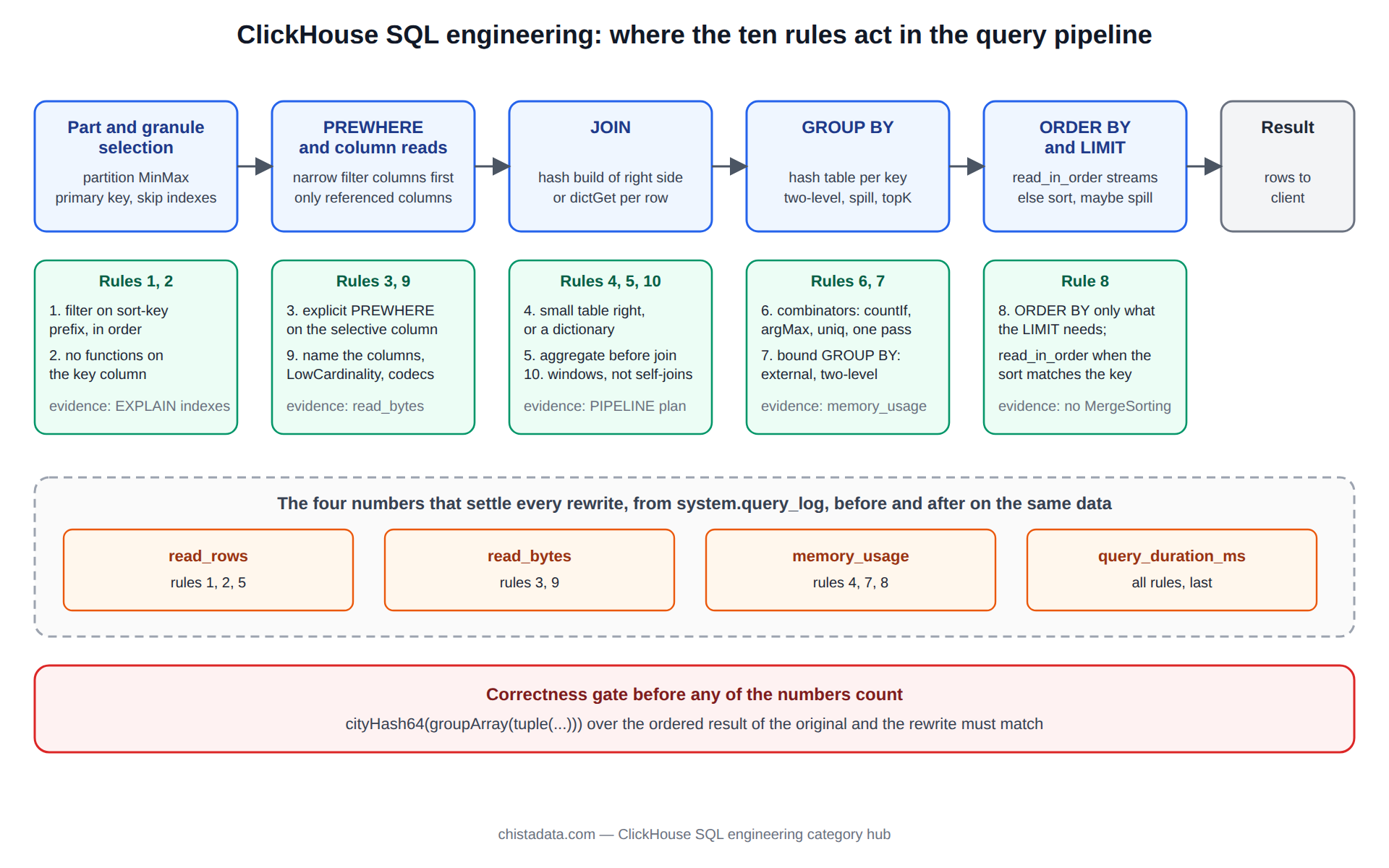
Every rule above is checked the same way. EXPLAIN indexes = 1 shows granules selected against total, which is rule one and two. EXPLAIN PIPELINE shows the transforms, which is where a join build, a sort step or a two-level aggregation is or is not present, for rules four, seven and eight. And system.query_log gives the four numbers that settle every argument: read_rows, read_bytes, memory_usage and query_duration_ms, before and after, on the same data.
The archive posts on the ClickHouse query optimizer and ClickHouse architecture and query performance explain what the optimiser does on its own so that the rules are applied where it does not.
| Rule | Symptom in the evidence | Fix |
|---|---|---|
| 1. Sort-key prefix | Granules selected close to total | Lead with the prefix column, or a projection |
| 2. No functions on key | Index not used despite key filter | Range on the raw column |
| 3. Explicit PREWHERE | read_bytes high for a selective query | PREWHERE the narrow selective column |
| 4. Small table right / dictionary | Memory limit on JoiningTransform | Swap sides, or dictGet |
| 5. Aggregate before join | Join input rows in the billions | Pre-aggregate subquery |
| 6. Combinators | Several scans of the same table | countIf, argMax, uniq in one pass |
| 7. Bounded GROUP BY | Memory limit exceeded on aggregation | External group by, two-level, topK |
| 8. Cheap ORDER BY | MergeSortingTransform on large input | read_in_order, reduce before sort |
| 9. Narrow columns | Bytes read far above rows × needed width | Column list, LowCardinality, codecs |
| 10. Windows over self-joins | Join of a table to itself | Window and array functions |
Settings that belong on the query, not in the profile
Several of the rules above lean on settings, and the temptation is to set them globally. Resist it. max_bytes_before_external_group_by, max_bytes_before_external_sort and a raised max_memory_usage are right for one heavy report and wrong for the dashboard user who shares the node; join_algorithm = 'grace_hash' or 'partial_merge' rescues one oversized join and slows every small one.
Attach them with a SETTINGS clause on the query, or on a settings profile scoped to the reporting user, and keep the default profile tight. The profile is a security boundary as much as a tuning surface, which the ClickHouse security hub covers under quotas and constraints.
Testing a rewrite without surprising anyone
A rewritten query must return the same rows as the original, and the proof is a checksum, not a glance. Run both forms with the same parameters, wrap each in SELECT cityHash64(groupArray(tuple(*))) over an ordered result, and compare the two hashes; a mismatch is a semantic change, most often from a JOIN that silently switched between inner and left, or from FINAL dropped on a ReplacingMergeTree.
Only after the hashes match do the four query_log numbers mean anything. Keep the original query and the rewrite together in version control with the hash check, because the next engineer to touch the dashboard will need to know why the query looks the way it does.
SELECT cityHash64(groupArray(tuple(country, category, revenue)))
FROM
(
    SELECT country, category, revenue
    FROM ( /* original or rewritten query here */ )
    ORDER BY country, category
);
Version notes
Window functions are stable since 21.x. optimize_read_in_order has been on by default since 20.x. The analyser, the new query planner, is the default since 24.3 and changes some EXPLAIN output and a handful of edge cases in aliasing; queries written against the old analyser should be re-checked on upgrade. The reference for the settings named here is the ClickHouse settings documentation; confirm the server version before relying on a default.
Reading the archive
Start with Rules for writing optimal SQL for ClickHouse performance and ClickHouse SQL engineering best practices, which are the long forms of the rules above, then the optimizer and execution-plan posts for the evidence side.
One more habit: keep a small corpus of the twenty slowest queries from system.query_log, refreshed monthly, and re-run the review against it after every ClickHouse upgrade. The optimiser improves in every release, and a rewrite that mattered on 24.x is sometimes done automatically on 26.x, which is worth knowing before the next engineer reapplies it by hand.
The rules are ordered by how often they pay off, not by difficulty. In practice rules one, two and nine account for most of the wins on a first review, because they are the ones a team migrating from a row store does not know to look for; rules four through seven are where the second review lives.
ChistaDATA’s ClickHouse consulting team runs query reviews against these ten rules with before-and-after numbers from the client’s own system.query_log, and 24×7 ClickHouse support takes the calls when a query that used to work stops fitting in memory. Test every rewrite against production-sized data on staging, compare the four query_log numbers, and only then change the dashboard or the application.