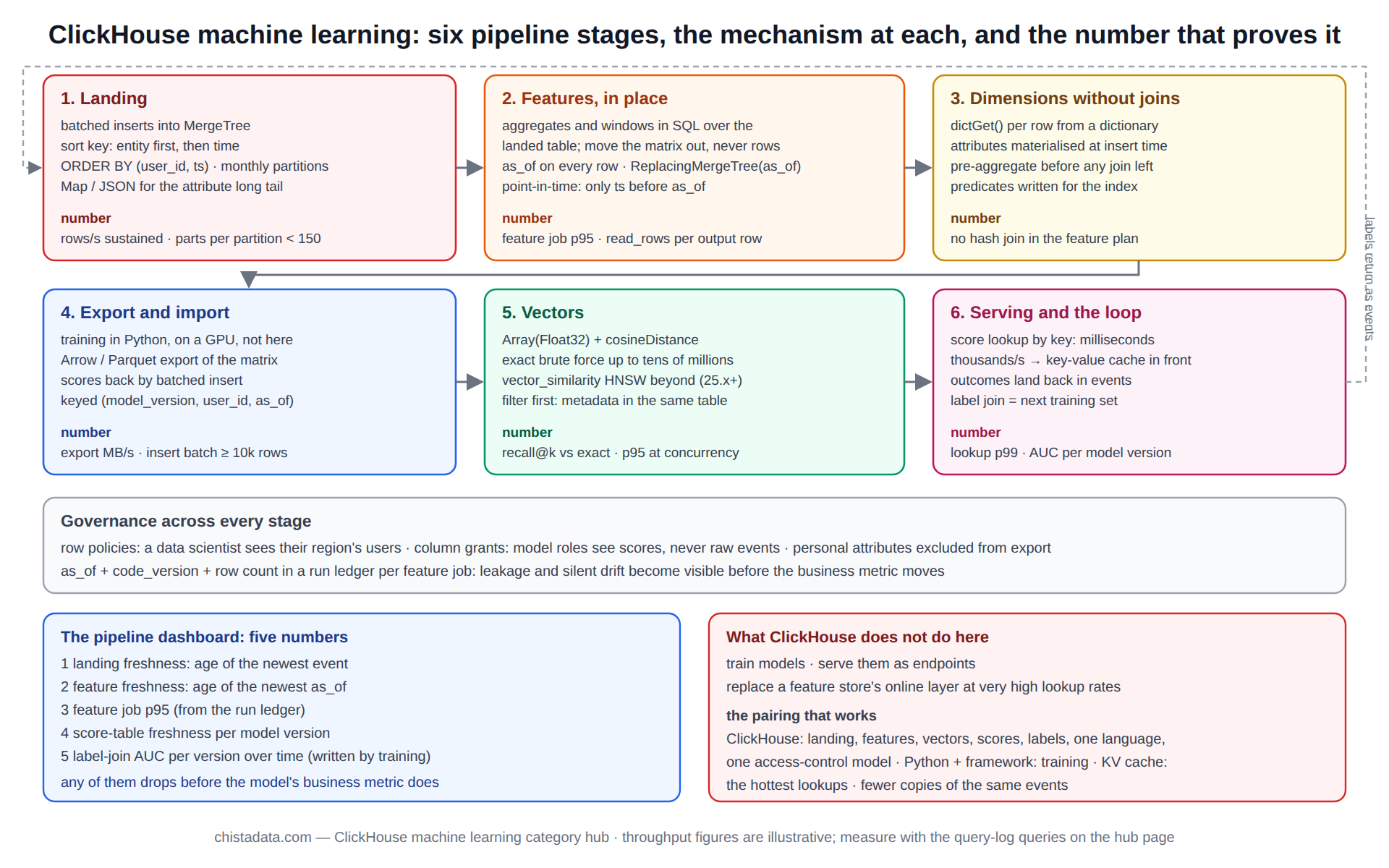
ClickHouse machine learning work rarely means training models inside the database. It means building the pipeline around the model on ClickHouse: landing raw events at high velocity, computing features in SQL over billions of rows in seconds, exporting training sets without copying the warehouse, storing embeddings and searching them, scoring in near real time, and governing who sees which rows. The model is the smallest part; the pipeline is where the engineering goes.
This page walks that pipeline as six stages, with the ClickHouse mechanism that carries each stage, the SQL that implements it, the number that says it is working, and the archive post that goes deeper. It is written for teams that already have a model and a warehouse and want to know what changes when the warehouse is ClickHouse.
The archive under this category holds the high-velocity ingestion and ETL posts, the fast data loops and dbt transformation posts, the join-elimination and criterion-indexability posts, the vector search and inverted-index posts, the ML-driven caching and ad-tech bid-tracking pipelines, data-level security, and compression for scale.
Stage 1: landing events at the rate the model needs
A ClickHouse machine learning pipeline starts where every ClickHouse pipeline starts: batched inserts of raw events into a MergeTree table with a sort key chosen for the feature queries that follow. The difference from a dashboard workload is volume and shape: feature computation reads wide windows over many entities, so the sort key leads with the entity (user, device, account) and then time, and partitioning stays monthly. The data ingestion built for high-velocity, high-volume post covers the insert path, and the optimising high-velocity ETL operations post covers the transformation step between landing and features.
CREATE TABLE events
(
    ts         DateTime64(3)          CODEC(Delta, ZSTD(1)),
    user_id    UInt64,
    event_type LowCardinality(String),
    amount     Float32,
    device     LowCardinality(String),
    attrs      Map(String, String)
)
ENGINE = ReplicatedMergeTree('/clickhouse/tables/{shard}/events', '{replica}')
PARTITION BY toYYYYMM(ts)
ORDER BY (user_id, ts);          -- entity first: feature windows read one user's rows contiguously

-- the number: rows per second sustained and parts per partition under 150
SELECT toStartOfMinute(event_time) AS m, sum(written_rows) / 60 AS rows_per_s
FROM system.query_log WHERE query_kind = 'Insert' AND type = 'QueryFinish' AND event_time > now() - INTERVAL 1 HOUR
GROUP BY m ORDER BY m;
Stage 2: ClickHouse machine learning features computed in SQL, in place
The reason to build ClickHouse machine learning pipelines at all is that features over billions of rows compute in seconds without moving data: rolling windows, per-entity statistics, sessionisation, funnel positions and ratios are aggregate functions and window functions over the landed table. The rule is to compute features in ClickHouse and move only the feature matrix out, never the raw rows. The building fast data loops post covers the iteration pattern where features are recomputed every few minutes, and the transforming data with dbt post shows the same logic managed as versioned models.
-- a feature matrix: 30-day behavioural features per user, one row per user
CREATE TABLE features_user_30d
(
    as_of        Date,
    user_id      UInt64,
    events_30d   UInt32,
    spend_30d    Float32,
    spend_p95    Float32,
    days_active  UInt8,
    kinds        UInt8,
    hours_since_last Float32,
    refund_rate  Float32
)
ENGINE = ReplacingMergeTree(as_of)
ORDER BY (user_id, as_of);

INSERT INTO features_user_30d
SELECT
    today()                                                    AS as_of,
    user_id,
    count()                                                    AS events_30d,
    sumIf(amount, event_type = 'purchase')                     AS spend_30d,
    quantileTDigestIf(0.95)(amount, event_type = 'purchase')   AS spend_p95,
    uniq(toDate(ts))                                           AS days_active,
    uniq(event_type)                                           AS kinds,
    dateDiff('hour', max(ts), now())                           AS hours_since_last,
    countIf(event_type = 'refund') / greatest(countIf(event_type = 'purchase'), 1) AS refund_rate
FROM events
WHERE ts >= now() - INTERVAL 30 DAY
GROUP BY user_id;
-- the number: feature job p95 in seconds, and read_rows per output row from system.query_log
Stage 3: joins, dictionaries and the shape of the feature query
Feature queries that join the fact table to five dimensions run outside the vectorised fast path and are the usual reason a feature job goes from seconds to minutes. The ClickHouse machine learning answer is the same as the analytics answer: dictionaries for small dimensions looked up per row, denormalised attributes materialised into the fact table at insert time, and pre-aggregation before any join that remains. The eliminating expensive joins post covers the three substitutions; the criterion indexability post covers writing feature predicates so that the primary index and skip indexes can serve them.
-- dimension lookups without a join
CREATE DICTIONARY user_dim
(
    user_id UInt64,
    segment String,
    country String,
    signup_date Date
)
PRIMARY KEY user_id
SOURCE(POSTGRESQL(host '${PG_HOST}' port 5432 user '${PG_USER}' password '${PG_PASSWORD}' db 'crm' table 'users'))
LAYOUT(HASHED())
LIFETIME(MIN 600 MAX 1200);

SELECT
    f.*,
    dictGet('user_dim', 'segment', f.user_id)                              AS segment,
    dateDiff('day', dictGet('user_dim', 'signup_date', f.user_id), f.as_of) AS tenure_days
FROM features_user_30d AS f
WHERE f.as_of = today();
Stage 4: exporting training sets and importing predictions
Training happens in Python, on a GPU or a cluster, not in ClickHouse; the pipeline’s job is to hand over the feature matrix efficiently and take the predictions back. The Python client streams Arrow or Parquet from a SELECT at hundreds of megabytes per second, which for a feature matrix of tens of millions of rows is a minute rather than an ETL job.
Predictions return by batched insert into a scores table keyed by entity and model version, from which the serving layer reads. The real-time bid tracking and optimisation post shows the loop in an ad-tech bid-tracking setting.
# export: the feature matrix as Arrow, straight into a DataFrame (clickhouse-connect)
import clickhouse_connect, os
client = clickhouse_connect.get_client(host=os.environ['CH_HOST'], username=os.environ['CH_USER'],
                                       password=os.environ['CH_PASSWORD'], secure=True)
df = client.query_df("SELECT * FROM features_user_30d WHERE as_of = today()")

# ... train, predict ...

# import: predictions back, batched, with the model version for lineage
client.insert('scores_user', rows, column_names=['as_of', 'user_id', 'model_version', 'score'])
CREATE TABLE scores_user
(
as_of Date,
user_id UInt64,
model_version LowCardinality(String),
score Float32
)
ENGINE = ReplacingMergeTree(as_of)
ORDER BY (model_version, user_id, as_of);
-- the number: export MB/s from the client log; import batch size ≥ 10k rows per insertStage 5: vectors, embeddings and similarity search in ClickHouse machine learning
Embeddings are Array(Float32) columns, and a similarity query is ORDER BY cosineDistance(embedding, query) LIMIT k. On tables up to tens of millions of rows a brute-force scan with the vectorised distance functions is fast enough and exact; beyond that the vector_similarity HNSW index (25.x and later, replacing the earlier annoy and usearch types) trades recall for latency.
Filtering before the distance (tenant, date, category) is what makes vector search on ClickHouse different from a dedicated vector store: the same table holds the metadata and the analytics. The ClickHouse for vector search and storage, part 2 post covers storage layout and the trade-offs, and the search hub compares vector, text and Bloom-filter mechanisms.
CREATE TABLE items
(
    item_id    UInt64,
    category   LowCardinality(String),
    updated    DateTime,
    embedding  Array(Float32)          -- 768 dims
)
ENGINE = MergeTree
ORDER BY (category, item_id);

-- exact, filtered: brute force over one category
SELECT item_id, cosineDistance(embedding, ${QUERY_VECTOR}) AS d
FROM items
WHERE category = 'footwear'
ORDER BY d ASC
LIMIT 20;

-- approximate, for the large unfiltered case (25.x+)
SET allow_experimental_vector_similarity_index = 1;
ALTER TABLE items ADD INDEX idx_emb embedding TYPE vector_similarity('hnsw', 'cosineDistance', 768) GRANULARITY 100000000;
-- the number: recall@20 against the exact query on a sample, and p95 latency at production concurrency
Stage 6: serving, caching and the feedback loop
Online scoring reads the scores table by entity key, which on a ReplacingMergeTree ordered by (model_version, user_id) is a primary-key lookup in milliseconds; at thousands of lookups per second it belongs in a key-value cache fed from ClickHouse rather than in ClickHouse itself. The archive’s intelligent caching with machine learning post turns the problem around and uses a model to decide what ClickHouse should cache. The feedback loop closes when outcomes (a purchase, a fraud confirmation, a click) land back in the events table and become next month’s labels.
-- the label join for the next training run: predictions against what happened
SELECT
    s.user_id,
    s.score,
    countIf(e.event_type = 'purchase') > 0                    AS converted
FROM scores_user AS s
LEFT JOIN events AS e
    ON e.user_id = s.user_id AND e.ts >= toDateTime(s.as_of) AND e.ts < toDateTime(s.as_of + 7)
WHERE s.model_version = 'v14' AND s.as_of = today() - 8
GROUP BY s.user_id, s.score;
-- the number: model AUC per version over time, stored in ClickHouse alongside the scores
Scheduling, backfills and point-in-time correctness
Feature jobs run on a schedule, and the two mistakes that break a ClickHouse machine learning model in production are both about time: computing features with data that arrived after the label (leakage) and recomputing history with today’s code but yesterday’s data gaps (silent drift). Keeping as_of in every feature and score table, computing features only from rows with ts < as_of, and storing each run’s version and row count make both detectable.
Backfills run partition by partition with the same query and a different as_of, and the ReplacingMergeTree key on (user_id, as_of) means a rerun replaces rather than duplicates.
-- point-in-time features: only rows that existed before the cut-off
INSERT INTO features_user_30d
SELECT toDate('2026-08-01') AS as_of, user_id, count() AS events_30d, /* … */
FROM events
WHERE ts >= toDateTime('2026-08-01') - INTERVAL 30 DAY AND ts < toDateTime('2026-08-01')
GROUP BY user_id
SETTINGS log_comment = 'features:backfill:2026-08-01';

-- run ledger: one row per feature run, checked before training starts
CREATE TABLE feature_runs
(
    as_of DateTime, job LowCardinality(String), code_version String, rows UInt64, duration_s Float32
)
ENGINE = MergeTree ORDER BY (job, as_of);
Watching the pipeline: five numbers on one dashboard
The platform’s own monitoring for a ClickHouse machine learning pipeline is five numbers: landing freshness (age of the newest event), feature freshness (age of the newest as_of), feature job p95, score-table freshness per model version, and the label-join AUC per version over time. The first four come from the tables and the query log; the fifth is written by the training job. A drop in any of them is visible before the model’s business metric moves, which is the point. The monitoring hub covers the cluster-level numbers underneath.
SELECT
    (SELECT dateDiff('minute', max(ts), now()) FROM events WHERE ts > now() - INTERVAL 1 DAY)    AS landing_lag_min,
    (SELECT dateDiff('hour', max(toDateTime(as_of)), now()) FROM features_user_30d)               AS feature_age_h,
    (SELECT max(model_version) FROM scores_user WHERE as_of = today())                             AS latest_scored_version,
    (SELECT quantile(0.95)(duration_s) FROM feature_runs WHERE as_of > now() - INTERVAL 7 DAY)   AS feature_p95_s;
Governance: who sees which rows in a ClickHouse machine learning platform
Feature tables contain the most sensitive view of a customer the company has, so row and column policies are part of the pipeline, not an afterthought: a data scientist sees features for their region’s users, a model service sees scores but not raw events, and personal attributes are masked or excluded from the export. ClickHouse row policies and column-level grants express this directly, and the data level security in ClickHouse post is the complete guide. The security hub covers the surrounding controls.
CREATE ROLE ds_emea;
GRANT SELECT(as_of, user_id, events_30d, spend_30d, spend_p95, days_active, kinds, refund_rate) ON features_user_30d TO ds_emea;
CREATE ROW POLICY emea_only ON features_user_30d
    FOR SELECT USING dictGet('user_dim', 'country', user_id) IN ('DE', 'FR', 'NL', 'ES', 'IT') TO ds_emea;

CREATE ROLE model_service;
GRANT SELECT ON scores_user TO model_service; -- scores, never events| Stage | ClickHouse mechanism | The number that says it works | Archive post |
|---|---|---|---|
| 1. Landing | batched inserts, entity-first sort key | rows/s sustained; parts per partition | high-velocity ingestion, ETL optimisation |
| 2. Features | aggregates and windows in SQL, in place | feature job p95; read_rows per output row | fast data loops, dbt |
| 3. Dimensions | dictionaries, materialised attributes | no hash join in the feature plan | eliminating joins, criterion indexability |
| 4. Export / import | Arrow export, batched score inserts | export MB/s; insert batch size | bid tracking pipelines |
| 5. Vectors | Array(Float32), cosineDistance, HNSW index | recall@k vs exact; p95 at concurrency | vector search part 2 |
| 6. Serving and loop | key lookups, cache, label join | lookup p99; AUC per model version | intelligent caching |
| Governance | row policies, column grants | zero raw-event access from model roles | data level security |
Sizing the pipeline: compression and the feature window
The raw event table dominates storage and the feature window dominates compute. Compression decides the first: typed columns, LowCardinality for categorical attributes and Delta codecs on timestamps routinely give 10× or more on event data, which is the difference between a feature window that fits the hot tier and one that does not. The data compression for performance and scalability post measures the options. The window decides the second: a 30-day feature job reads 30 days of one entity’s rows per entity, and with an entity-first sort key that is a sequential read per user rather than a scan.
-- what the feature job costs, per run, from the query log
SELECT
    log_comment,
    quantile(0.95)(query_duration_ms) / 1000        AS p95_s,
    formatReadableQuantity(avg(read_rows))          AS rows_read,
    formatReadableQuantity(avg(result_rows))        AS rows_out,
    round(avg(read_rows) / avg(result_rows))        AS rows_read_per_feature_row,
    formatReadableSize(max(memory_usage))           AS peak_mem
FROM system.query_log
WHERE type = 'QueryFinish' AND log_comment LIKE 'features:%' AND event_time > now() - INTERVAL 7 DAY
GROUP BY log_comment;
What ClickHouse machine learning does not do
ClickHouse does not train models, serve them as endpoints, or replace a feature store’s online layer at very high lookup rates, and a design that asks it to do any of those will be slower than the purpose-built tool. Its part of the pipeline is the batch and near-real-time data layer: landing, features, vectors, scores and labels, all queryable with one language and one set of access controls. The pairing that works is ClickHouse for that layer, Python and the training framework for models, and a key-value cache in front for the hottest lookups.
The boundary matters commercially as much as technically: teams that buy a feature store and a vector database and a warehouse for one model usually end up with three copies of the same events and three access-control models. Consolidating the batch and near-real-time layer on ClickHouse removes two of the copies; the remaining specialised tools then hold only what they are good at.
Version notes
The vector_similarity index replaced annoy and usearch in 25.x; the archive’s vector post predates it and its index syntax needs updating. Row policies and column grants have been stable since 20.x. quantileTDigest and the -If combinators used in the feature query have been available since 19.x. The clickhouse-connect documentation is the source for the Python export and insert calls; confirm the client version against the running server.
Reading the archive
The posts below were written across three years and two LTS generations; the pipeline order is the reading order, and the version notes above flag where syntax has since moved.
Read in stage order. Landing: the high-velocity ingestion and ETL optimisation posts. Features: fast data loops and dbt. Dimensions and query shape: eliminating expensive joins and criterion indexability. Export and loops: the bid-tracking pipeline. Vectors: vector search part 2 and the inverted-index post for text features. Serving: intelligent caching with ML. Governance and sizing: data level security and compression for scalability.
ChistaDATA builds this pipeline as a ClickHouse consulting engagement, usually alongside a customer’s existing data science team, and runs the data layer under managed services with the feature-job and freshness numbers above as standing alerts. Test every stage on staging with production-shaped data, keep the raw events table backed up with a tested restore, and never grant a model role access to rows it does not need.