Troubleshooting High CPU Usage in ClickHouse: From system.trace_log to Flamegraphs

Sustained ClickHouse high CPU usage is one of the few symptoms where system.query_log alone cannot finish the diagnosis: it tells you which queries burned CPU, but not where inside the engine the cycles went. That answer lives in system.trace_log, populated by ClickHouse’s built-in sampling profiler, and it renders best as a flamegraph. This post walks the full production workflow we use at ChistaDATA — enabling the profiler safely, extracting and symbolizing stacks, generating flamegraphs, and reading the recurring CPU hotspot patterns — for engineers who need to answer “why is this box at 90% CPU” with a function name, not a guess.

Treat what follows as a runbook rather than a reference: each step is a checkpoint you can finish in minutes, and together they convert a vague ClickHouse high CPU usage ticket into a named function on a flamegraph. Everything runs on 100% open-source ClickHouse using tables the server already ships, so every ClickHouse high CPU usage investigation below is reproducible without an agent, a sidecar, or a vendor-specific build.

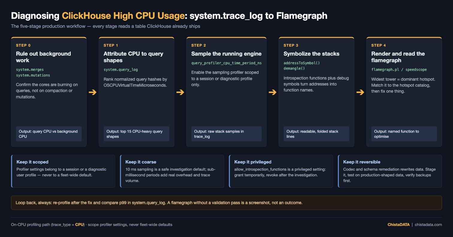
Step 0 — Confirm It’s Actually Query CPU

Before profiling queries, rule out the two background consumers that routinely masquerade as query load. Merges: SELECT count(), sum(rows_read) FROM system.merges; — a compaction storm after heavy inserts is CPU-intensive by design. Mutations: SELECT count() FROM system.mutations WHERE is_done = 0; — part rewrites from ALTER ... UPDATE/DELETE burn the same cores. Then attribute the remainder to query shapes via query_log:

SELECT
    normalized_query_hash,
    any(query)                                                    AS sample_query,
    count()                                                       AS executions,
    sum(ProfileEvents['OSCPUVirtualTimeMicroseconds']) / 1e6      AS total_cpu_s,
    sum(query_duration_ms) / 1e3                                  AS total_wall_s
FROM system.query_log
WHERE type = 'QueryFinish'
  AND event_time >= now() - INTERVAL 1 HOUR
GROUP BY normalized_query_hash
ORDER BY total_cpu_s DESC
LIMIT 15;

OSCPUVirtualTimeMicroseconds is actual CPU time consumed, so total_cpu_s materially above total_wall_s confirms heavy intra-query parallelism — the query shapes at the top of this list are your profiling targets.

Only once merges and mutations are ruled out should the incident be handled as a query-level ClickHouse high CPU usage problem — otherwise you will tune SQL while a compaction backlog keeps the cores busy. If part counts are the real story, the fix lives in MergeTree sort keys, partitioning and insert batching, not in the profiler.

Step 1 — Enable the Sampling Profiler (Scoped, Not Global)

The sampling profiler (documented in the official sampling query profiler guide) writes stack samples into system.trace_log. The knobs are per-query settings, so enable them for your investigation session or a targeted user profile rather than server-wide:

SET query_profiler_cpu_time_period_ns  = 10000000;   -- 10 ms CPU-time sampling
SET query_profiler_real_time_period_ns = 10000000;   -- 10 ms wall-time sampling (catches off-CPU waits)

-- Run the suspect query, tagged for easy retrieval:
SELECT /* cpu_probe */ ...
SETTINGS log_comment = 'cpu_probe_2026_07_30';

Notes from production use: 10 ms periods are a reasonable investigation default — aggressive periods (≤1 ms) add measurable overhead and trace volume, so treat them as short-lived diagnostics, never a permanent fleet setting. In many recent builds the CPU profiler is active by default at a coarse period; verify what is actually in effect on your version with SELECT name, value, changed FROM system.settings WHERE name LIKE 'query_profiler%'; rather than assuming. Behavior here is version-sensitive across the 22.x–24.x line, and self-managed open-source ClickHouse gives you full access to trace_log, whereas managed/cloud offerings may restrict introspection surface — confirm before you depend on it.

Scoping is not a detail. A fleet-wide profiler setting turns a temporary ClickHouse high CPU usage investigation into a permanent tax on every query, which is exactly the outcome you are trying to avoid.

Step 2 — Symbolize Stacks from system.trace_log

trace_log stores raw instruction addresses; the introspection functions addressToSymbol and demangle convert them to readable frames. They require allow_introspection_functions = 1 (a privileged setting — grant it to the investigating user only, temporarily, and revoke after) and the clickhouse-common-static-dbg debug-symbol package on the host for line-level detail:

SET allow_introspection_functions = 1;

SELECT
    count()                                                   AS samples,
    arrayStringConcat(
        arrayMap(addr -> demangle(addressToSymbol(addr)), trace),
        ';'
    )                                                         AS stack
FROM system.trace_log
WHERE trace_type = 'CPU'
  AND event_time >= now() - INTERVAL 30 MINUTE
  AND query_id IN
  (
      SELECT query_id
      FROM system.query_log
      WHERE log_comment = 'cpu_probe_2026_07_30'
        AND type = 'QueryFinish'
  )
GROUP BY stack
ORDER BY samples DESC
LIMIT 40;

trace_type = 'CPU' isolates on-CPU samples; the same table also holds 'Real' (wall-clock) samples and, since ClickHouse 22.x+, memory-related trace types — useful later, but noise for a CPU hunt.

Symbolization is what makes a ClickHouse high CPU usage report actionable: without debug symbols you are left with raw addresses no engineer can act on, and with them you get function names your team can map back to schema, codec, or query decisions.

Step 3 — Render the Flamegraph

The semicolon-joined stack format above is exactly what Brendan Gregg’s flamegraph.pl consumes. Export and render:

clickhouse-client \
    --user ${CH_USER} --password ${CH_PASSWORD} \
    --query "
SELECT
    arrayStringConcat(arrayMap(addr -> demangle(addressToSymbol(addr)), trace), ';') AS stack,
    count() AS samples
FROM system.trace_log
WHERE trace_type = 'CPU'
  AND event_date = today()
GROUP BY stack
FORMAT TabSeparated" \
    --allow_introspection_functions 1 \
> stacks.folded

flamegraph.pl --title "clickhouse CPU $(date +%F)" stacks.folded > ch_cpu.svg

Alternatives that read the same folded format: speedscope (drag-and-drop, better for sharing with app teams) and Grafana’s flamegraph panel if you already ship trace_log into observability storage. Whatever the renderer, the reading discipline is identical: width = share of samples = share of CPU; look at the widest towers first and read them bottom-up to find the deepest frame that is still wide.

Keep the folded stack file. Attaching it to the incident ticket lets the next engineer reproduce your ClickHouse high CPU usage finding instead of trusting a picture.

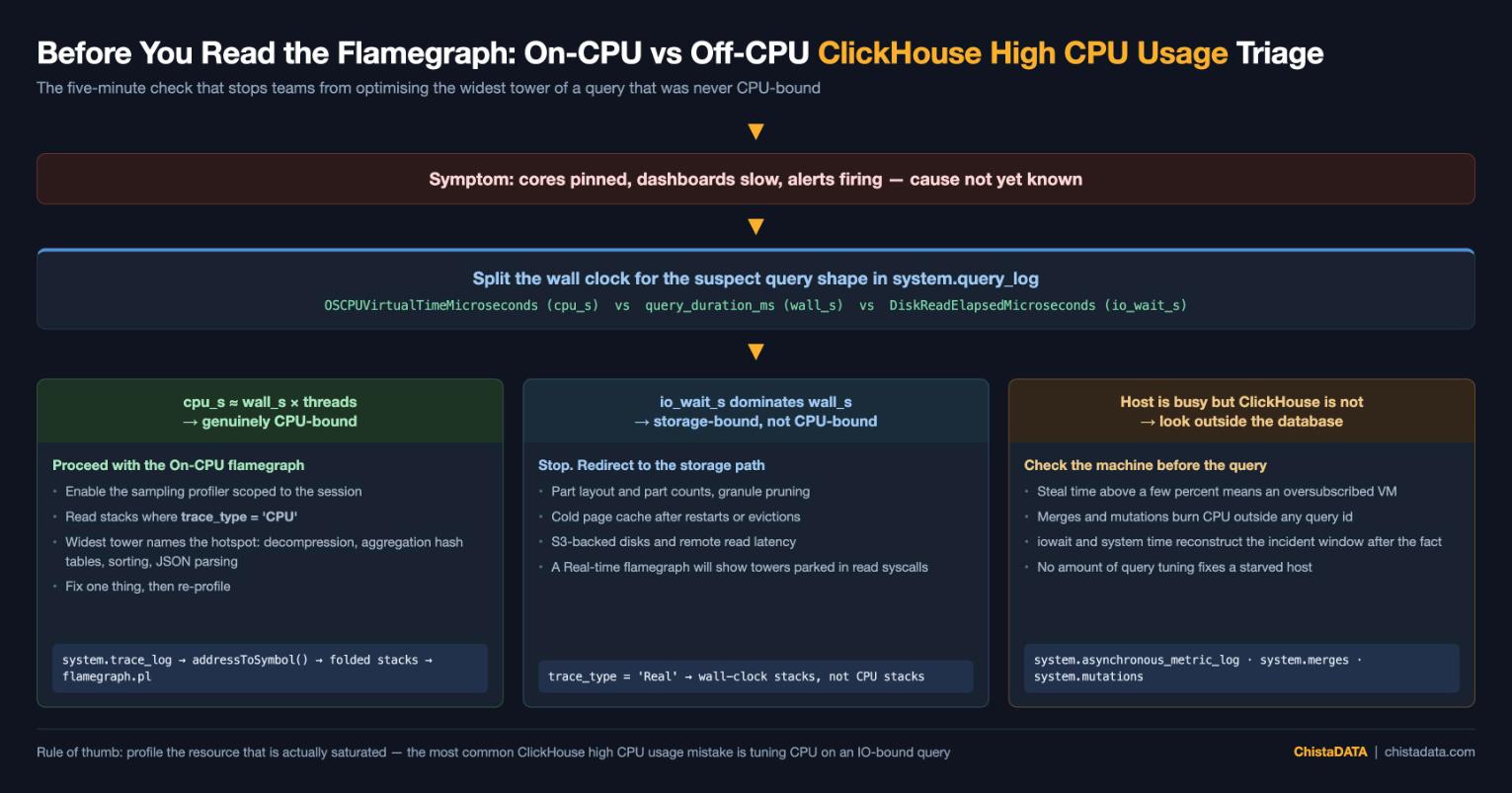
Step 3.5 — On-CPU vs Off-CPU: The Comparison That Prevents Wrong Conclusions

The reason to sample both trace_type = 'CPU' and trace_type = 'Real' is that their difference is the wait profile. A query with 40 s wall-clock and 6 s of CPU samples is not a CPU problem no matter what the flamegraph’s widest tower says — 85% of its life was spent off-CPU on IO, locks, or the network. Quantify the split per query before interpreting any flamegraph:

SELECT
    trace_type,
    count()                        AS samples
FROM system.trace_log
WHERE query_id = ${TARGET_QUERY_ID}
GROUP BY trace_type;

-- Cross-check against wall clock and CPU time from query_log:
SELECT
    query_duration_ms / 1e3                                       AS wall_s,
    ProfileEvents['OSCPUVirtualTimeMicroseconds'] / 1e6           AS cpu_s,
    ProfileEvents['OSIOWaitMicroseconds'] / 1e6                   AS io_wait_s,
    ProfileEvents['DiskReadElapsedMicroseconds'] / 1e6            AS disk_read_s
FROM system.query_log
WHERE query_id = ${TARGET_QUERY_ID}
  AND type = 'QueryFinish';

Decision rule: cpu_s ≈ wall_s × threads means genuinely CPU-bound — proceed with the CPU flamegraph. io_wait_s dominating redirects the investigation to storage (part layout, cold page cache, S3-backed disks), where a Real-time flamegraph will show the towers sitting in read syscalls instead. This five-minute check regularly saves days: the single most common profiling mistake we see in the field is optimizing the widest CPU tower of a query that was IO-bound all along.

For host-level context around the incident window, system.asynchronous_metric_log retains OS-level CPU counters (user, system, iowait, steal — the latter matters on oversubscribed VMs) on an interval, letting you reconstruct whether the machine was saturated even after the moment has passed. Steal time above a few percent on cloud instances is its own diagnosis and no amount of query tuning will fix it.

Getting this comparison right is the difference between fixing ClickHouse high CPU usage and rewriting a query that was never CPU-bound in the first place. The wider set of counters worth watching alongside the profiler is covered in our ClickHouse performance observability and monitoring whitepaper.

Step 4 — The ClickHouse High CPU Usage Hotspot Catalog

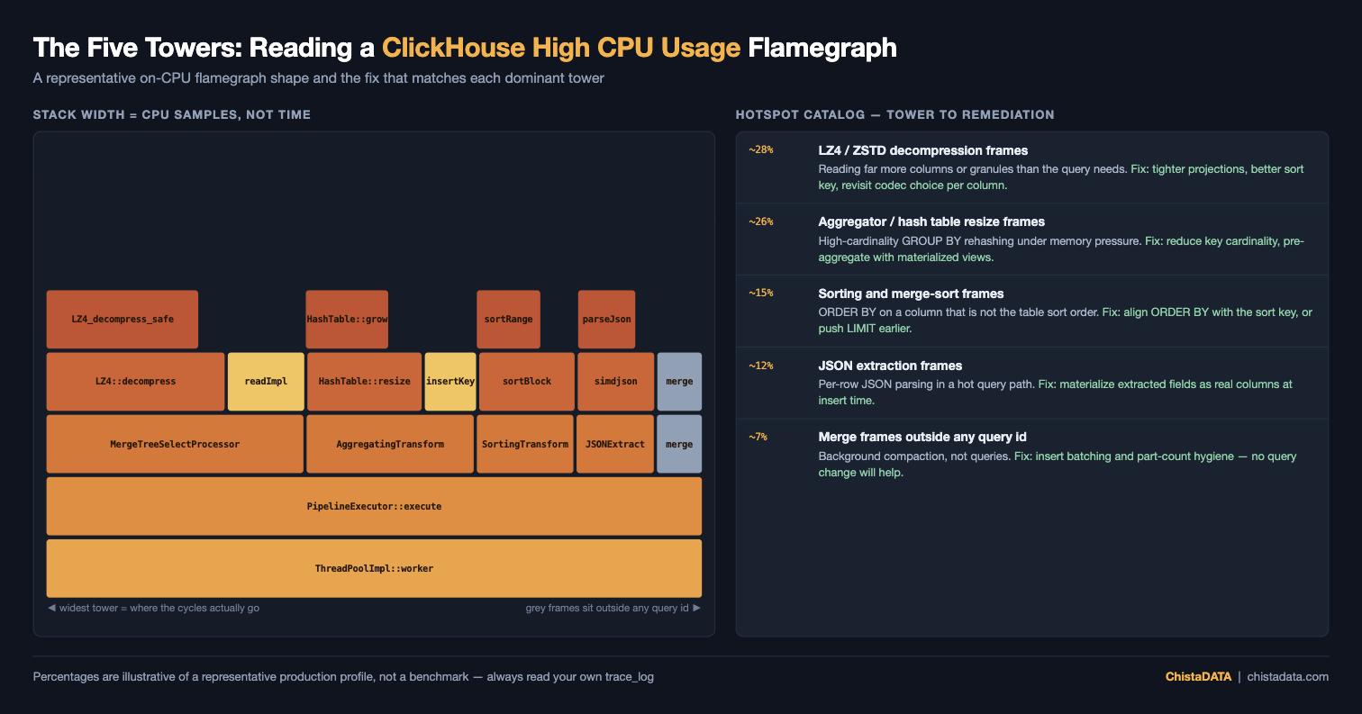
Most ClickHouse high CPU usage investigations resolve to a small set of recognizable towers. What each one means, and the measured next step:

Anonymized field example: a SaaS analytics customer’s cluster pinned all cores every morning; query_log blamed a modest-looking dashboard query. The flamegraph showed the width concentrated in JSON extraction frames — the query parsed a raw JSON column per row, per request. Materializing three extracted columns at ingest moved the work from query time to insert time; the fix was validated by re-profiling and by the p99 drop in query_log, not by feel.

Five patterns cover the overwhelming majority of ClickHouse high CPU usage cases we see in the field, so match your widest tower against the catalog above before inventing a new theory. For a broader triage grid across query and IOPS symptoms, see our ClickHouse troubleshooting matrices.

Step 5 — Validate the Fix the Same Way You Found the Problem

A CPU fix is proven by three measurements converging, all from tables already used above: the flamegraph tower you targeted shrinks proportionally on a re-profile of the same query shape; ProfileEvents['OSCPUVirtualTimeMicroseconds'] per execution drops in query_log for that normalized_query_hash; and host CPU utilization in system.asynchronous_metric_log falls across the same daily window that was previously saturated. If only the flamegraph changed, you moved the work, not removed it — JSON materialization, for example, shifts cycles from query time to insert time, and the insert pipeline’s CPU budget must absorb them, which the second measurement will reveal.

Two environment caveats worth stating for modern fleets. In containers, CPU limits are cgroup-enforced: a pod throttled at 8 cores reports throttling in cgroup stats while ClickHouse happily schedules max_threads = 32 workers against it — check container CPU quota against effective max_threads before concluding the engine is inefficient. And on shared cloud instances, steal time from system.asynchronous_metric_log belongs in every CPU investigation summary, because a correct query fix on a stolen-CPU host produces a disappointing before/after and erodes trust in the whole methodology.

Standard caveats apply with extra force here: introspection settings are privileged, debug-symbol packages change host footprint, and remediation (codec changes, schema materialization) rewrites data. Test everything in a staging environment against production-shaped data before production rollout, stage changes reversibly, and keep your backup/DR posture verified before any schema or codec migration.

Re-profiling closes the loop. If the tower you targeted did not shrink, the real ClickHouse high CPU usage root cause is still in the cluster, and the next change should be guided by a fresh flamegraph rather than by the previous hypothesis.

Key Takeaways

• Rule out merges (system.merges) and mutations (system.mutations) before blaming queries — background compaction is a top cause of ClickHouse high CPU usage, and no query fix touches it.
• Attribute ClickHouse high CPU usage to query shapes with ProfileEvents['OSCPUVirtualTimeMicroseconds'] in query_log, then profile only the top shapes.
• Enable query_profiler_cpu_time_period_ns scoped to a session or profile; verify effective profiler settings per version in system.settings instead of assuming defaults.
• Symbolize system.trace_log stacks with addressToSymbol + demangle (requires allow_introspection_functions = 1 and debug symbols), and render with flamegraph.pl or speedscope.
• Most ClickHouse high CPU usage flamegraphs resolve to five towers — decompression, aggregation hash tables, sorting, JSON parsing, or background merges — each with a distinct, measurable fix.
• Close the loop: re-profile and compare query_log p99 after the fix; a flamegraph without a validation pass is a screenshot, not an outcome.
• Treat ClickHouse high CPU usage as a measurement problem before a tuning problem: profile, change one thing, then re-profile to prove the change worked.

FAQ

Why is ClickHouse using 100% CPU?

The three usual sources of ClickHouse high CPU usage are background merges after heavy inserts, running mutations, and CPU-heavy query shapes (decompression, high-cardinality aggregation, JSON parsing). Check system.merges and system.mutations first, then rank queries by OSCPUVirtualTimeMicroseconds in system.query_log.

How do I profile CPU usage of a ClickHouse query?

Set query_profiler_cpu_time_period_ns for the session, run the query with a log_comment tag, then read its stacks from system.trace_log (trace_type = 'CPU') symbolized via demangle(addressToSymbol(...)).

How do I generate a flamegraph from ClickHouse?

Aggregate trace_log stacks into semicolon-joined folded format with sample counts, export as TabSeparated, and feed the file to flamegraph.pl or open it in speedscope. Debug-symbol packages on the host give readable, line-accurate frames.

Does the ClickHouse query profiler slow down production?

At coarse sampling periods (around 10 ms) the overhead is small for investigation windows; aggressive sub-millisecond periods add measurable cost and trace volume. Scope profiler settings to sessions or a diagnostic profile rather than server-wide defaults, and verify effective values in system.settings.

How do I fix ClickHouse high CPU usage quickly?

There is no single switch. The fastest reliable path is the sequence above: separate background work from query work, rank query shapes by actual CPU time, profile only the top shapes, then read the flamegraph. In practice most ClickHouse high CPU usage incidents are closed by one targeted change — a codec swap, a lower-cardinality GROUP BY, materialized JSON fields, or insert batching to calm merges.

Does adding CPU cores fix ClickHouse high CPU usage?

Rarely, and never permanently. More cores hide the symptom while the per-row cost stays the same, so the same ClickHouse high CPU usage pattern returns as data volume grows. Profile first, remove the hot work, and scale afterwards only if the flamegraph shows the remaining cost is genuinely parallel and unavoidable.

When ClickHouse high CPU usage is costing you SLAs right now, ChistaDATA’s ClickHouse Performance Consulting and 24x7x365 Support runs this exact profiling workflow on production clusters under a 15-minute S1 response SLA — on 100% open-source ClickHouse, zero vendor lock-in. Get a ChistaDATA engineer on your cluster.