ClickHouse query performance is decided by the shape of the statement more than by any server setting, because the engine does exactly what the SQL asks: it reads the columns named, in the granules the predicates allow, through the operators the clauses imply. A query that names three columns instead of thirty, filters on the sort key instead of a function of it, and aggregates a pre-reduced set instead of raw rows is faster by orders of magnitude on the same hardware with the same configuration.
This page is a catalogue of the rewrites that produce those orders of magnitude, each shown as a before-and-after pair with the plan evidence that proves the difference, so that the pattern can be recognised in a query log and applied without guesswork.
The performance hub covers the system-level review; this page is the query-level companion. The archive posts go deeper on individual patterns: PREWHERE versus WHERE, LowCardinality, the fan trap, partitioning for query speed, stuck queries and the query optimizer.
Pattern 1: name the columns, because ClickHouse query performance is paid per column
The most common regression in a ClickHouse query log is SELECT * from a wide table feeding an application that uses four fields. Every column named is a file opened, decompressed and moved through the pipeline; on a 60-column table with String payloads, the difference between four columns and sixty is the difference between reading 200 MB and 8 GB for the same rows.
-- before: 60 columns read, 8.1 GB, 4.2 s (illustrative)
SELECT *
FROM events
WHERE event_date = today() AND tenant_id = 42;

-- after: 4 columns read, 210 MB, 0.3 s
SELECT event_time, event_type, user_id, amount_cents
FROM events
WHERE event_date = today() AND tenant_id = 42;

-- evidence: read_bytes and read_columns in system.query_log for the two shapes
Pattern 2: filter on the sort key as stored, not on a function of it
The primary index holds the raw sort-key values, so a predicate that wraps the key column in a function (toDate(ts) = '2026-09-01', lower(status) = 'ok', ts + INTERVAL 1 HOUR > now()) usually cannot use it and reads every granule. Rewriting the predicate as a range on the raw column restores pruning. ClickHouse can push some monotonic functions through the index (toDate, toStartOfDay on a DateTime key are handled since 20.x), but the safe rule for ClickHouse query performance is to compare the stored column against constants.
-- before: PrimaryKey Granules 61440/61440 (nothing pruned)
SELECT count() FROM events
WHERE toYYYYMM(ts) = 202609 AND lower(status) = 'failed';

-- after: PrimaryKey Granules 512/61440
SELECT count() FROM events
WHERE ts >= toDateTime('2026-09-01 00:00:00')
  AND ts <  toDateTime('2026-10-01 00:00:00')
  AND status = 'failed';               -- store status lower-cased, or add a materialized lower(status)

-- evidence: EXPLAIN indexes = 1, PrimaryKey line before and after
Pattern 3: PREWHERE the cheap selective column for ClickHouse query performance
ClickHouse moves predicates into PREWHERE automatically (optimize_move_to_prewhere, on by default), reading the filter columns first and the rest only for rows that pass. The automatic choice is usually right, but on a table where the selective column is small and the expensive columns are wide, an explicit PREWHERE on the selective column can cut read bytes further, and on a query whose predicate is on a wide column the automatic move can make things worse. The PREWHERE versus WHERE post measures both cases.
-- before: WHERE on a wide JSON column reads the column for every row in the granule
SELECT user_id, payload
FROM events
WHERE JSONExtractString(payload, 'kind') = 'refund' AND event_date = today();

-- after: cheap selective column in PREWHERE, wide column read only for survivors
SELECT user_id, payload
FROM events
PREWHERE event_type = 'refund'
WHERE event_date = today();

-- evidence: ProfileEvents['SelectedBytes'] and read_bytes; ideally materialize event_type
Pattern 4: LowCardinality and typed columns instead of String comparisons
A String column with a few hundred distinct values compares byte-by-byte on every row; the same column as LowCardinality(String) compares dictionary indexes and compresses far better. ClickHouse query performance on GROUP BY and WHERE over such columns improves several-fold from the type change alone, and the complete guide to LowCardinality post covers the thresholds (under roughly 10,000 distinct values is the usual rule) and the cases where it hurts.
-- schema-level rewrite; the query stays the same
ALTER TABLE events MODIFY COLUMN status LowCardinality(String);
ALTER TABLE events MODIFY COLUMN country  LowCardinality(String);
-- applies to new parts; MATERIALIZE COLUMN or wait for merges for old parts

-- same applies to UUIDs stored as String → UUID, timestamps as String → DateTime64
-- evidence: system.columns data_compressed_bytes and query_duration_ms for the GROUP BY shape
Pattern 5: aggregate before joining, and put the small side on the right
The default hash join builds the right-hand table in memory and streams the left through it. A join that puts the big fact table on the right builds a hash table the size of the fact table, and a join performed before aggregation multiplies rows through the join before reducing them. The rewrite is to aggregate each side to the join key first, then join the small results, and to keep the smaller relation on the right. The fan trap post covers the correctness side of the same mistake: a one-to-many join before sum() inflates the total silently.
-- before: 800M-row fact table on the right, joined then aggregated, MEMORY_LIMIT_EXCEEDED
SELECT c.segment, sum(e.amount_cents)
FROM customers AS c
JOIN events AS e ON e.customer_id = c.customer_id
WHERE e.event_date >= today() - 30
GROUP BY c.segment;

-- after: aggregate the fact table first, join 2M rows to 2M rows, small side right
SELECT c.segment, sum(agg.cents)
FROM
(
    SELECT customer_id, sum(amount_cents) AS cents
    FROM events
    WHERE event_date >= today() - 30
    GROUP BY customer_id
) AS agg
JOIN customers AS c ON c.customer_id = agg.customer_id
GROUP BY c.segment;

-- evidence: memory_usage and query_duration_ms; EXPLAIN PIPELINE shows the join build side
Join order matters on every engine, but on ClickHouse the asymmetry is larger because the build side is fully materialised before the first output row. For a small dimension that many queries join, a dictionary (dictGet) replaces the join entirely and is the fastest form of lookup ClickHouse has; for a very large right side, join_algorithm = 'grace_hash' or 'partial_merge' trades speed for bounded memory.
Pattern 6: pre-aggregate with a materialized view, the largest ClickHouse query performance win for repeated shapes
A dashboard that asks the same GROUP BY over the last day every thirty seconds is reading and aggregating the same rows every thirty seconds. A materialized view with AggregatingMergeTree maintains the aggregate at insert time, and the dashboard query reads the small target table with -Merge combinators. ClickHouse query performance for the repeated shape goes from seconds to milliseconds, and the cost moves to the insert path where it is amortised. The materialized view hub has the design rules; the pattern below is the minimum.
CREATE TABLE events_by_minute
(
    minute      DateTime,
    tenant_id   UInt32,
    event_type  LowCardinality(String),
    cnt         AggregateFunction(count),
    cents       AggregateFunction(sum, Int64),
    users       AggregateFunction(uniq, UInt64)
)
ENGINE = AggregatingMergeTree
PARTITION BY toYYYYMM(minute)
ORDER BY (tenant_id, event_type, minute);

CREATE MATERIALIZED VIEW events_by_minute_mv TO events_by_minute AS
SELECT
    toStartOfMinute(event_time) AS minute,
    tenant_id,
    event_type,
    countState()                AS cnt,
    sumState(amount_cents)      AS cents,
    uniqState(user_id)          AS users
FROM events
GROUP BY minute, tenant_id, event_type;

-- the dashboard query, now over a table hundreds of times smaller
SELECT
    toStartOfHour(minute) AS hour,
    countMerge(cnt)       AS events,
    sumMerge(cents) / 100 AS revenue,
    uniqMerge(users)      AS users
FROM events_by_minute
WHERE tenant_id = 42 AND minute >= now() - INTERVAL 1 DAY
GROUP BY hour
ORDER BY hour;
Pattern 7: approximate where exact is not required
uniqExact holds every distinct value in memory; uniq (HyperLogLog-based, error around 1 to 2 percent) holds a fixed sketch. quantileExact sorts; quantileTDigest or quantile (reservoir) do not. For dashboards and trend lines the approximate forms are the right ClickHouse query performance choice and the exact forms are reserved for reconciliation, where the number must match another system. The change is one function name and the memory difference on a high-cardinality column is often the difference between finishing and MEMORY_LIMIT_EXCEEDED.
-- before: uniqExact over 400M user_id values, 12 GB of hash table
SELECT toDate(event_time) AS d, uniqExact(user_id) FROM events WHERE event_date >= today() - 90 GROUP BY d;

-- after: uniq, fixed ~ 100 KB per group, same trend line
SELECT toDate(event_time) AS d, uniq(user_id) FROM events WHERE event_date >= today() - 90 GROUP BY d;

-- evidence: memory_usage in system.query_log; uniqCombined64 when a lower error is needed
Pattern 8: LIMIT BY, argMax and ASOF JOIN instead of self-joins and subqueries
Three questions that produce slow self-joins in other dialects have direct forms in ClickHouse, and using them is one of the cheapest improvements available. “Latest row per key” is argMax(col, ts) or LIMIT 1 BY key with ORDER BY ts DESC, not a join to a max(ts) subquery. “Top N per group” is LIMIT N BY group. “Nearest earlier row in another table” is ASOF JOIN, not a correlated subquery with max(). Each rewrite removes a full pass over the table, and the optimize ClickHouse queries post has more of them, each with the read_rows evidence.
-- before: latest status per order via self-join, two scans and a hash table
SELECT o.order_id, o.status
FROM order_events AS o
JOIN (SELECT order_id, max(ts) AS ts FROM order_events GROUP BY order_id) AS m
  ON m.order_id = o.order_id AND m.ts = o.ts;

-- after: one scan
SELECT order_id, argMax(status, ts) AS status
FROM order_events
GROUP BY order_id;

-- or, keeping whole rows:
SELECT * FROM order_events ORDER BY order_id, ts DESC LIMIT 1 BY order_id;
Pattern 9: shape the query to the distributed plan
On a cluster, a GROUP BY over a Distributed table runs in two stages: each shard aggregates locally, the initiator merges. A high-cardinality key makes the merge the bottleneck; a subquery in IN or a join against a non-replicated table makes every shard re-execute it.
The rewrites are GLOBAL IN and GLOBAL JOIN for the subquery case, distributed_group_by_no_merge or a sharding key aligned with the group key for the cardinality case, and optimize_skip_unused_shards = 1 so that a predicate on the sharding key sends the query to one shard. The sharding archive covers the design side; the ClickHouse query performance side is recognising which of the three the query log is showing.
Pattern 10: bound the query, so ClickHouse query performance failures are cheap
The last pattern is not a rewrite but a wrapper. A query with no max_execution_time, no max_rows_to_read and no max_result_rows can take the cluster’s memory and time with it; a query with all three fails early and cheaply when its shape is wrong.
Setting them per profile (dashboard users at 30 s and 1 billion rows, batch users higher, ad-hoc users lowest) means the patterns above are enforced by the limits: a query that reads every granule because it violates pattern 2 hits max_rows_to_read before it hurts anyone, and the exception in system.query_log is the ticket that gets it rewritten.
-- per-profile bounds, users.xml or SQL-managed profile (illustrative values)
CREATE SETTINGS PROFILE dashboard_profile SETTINGS
    max_execution_time = 30,
    max_rows_to_read = 1000000000,
    max_result_rows = 100000,
    max_memory_usage = 8000000000,
    max_threads = 8;
ALTER USER ${CH_DASHBOARD_USER} SETTINGS PROFILE 'dashboard_profile';
Query-level SETTINGS clauses can loosen a bound for one known-heavy statement without changing the profile, which keeps the exception for the rest. The performance settings post lists the current defaults for each.
Reading the plan: the ClickHouse query performance evidence for every rewrite
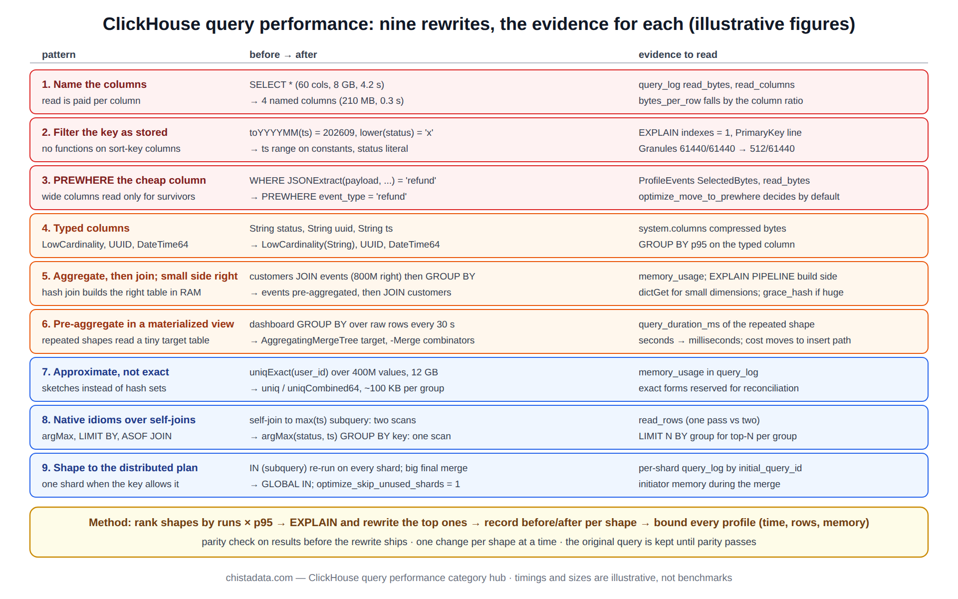
| Pattern | What to read | Before | After |
|---|---|---|---|
| 1. Columns | query_log read_bytes, read_columns | GB, dozens of columns | MB, the columns used |
| 2. Key predicates | EXPLAIN indexes = 1 PrimaryKey line | all granules | a few percent |
| 3. PREWHERE | ProfileEvents SelectedBytes | wide column read for all rows | read for survivors |
| 4. Types | system.columns compressed bytes; GROUP BY p95 | String | LowCardinality, UUID, DateTime |
| 5. Joins | memory_usage; EXPLAIN PIPELINE build side | fact table on right | aggregated, small side right |
| 6. Pre-aggregation | query_duration_ms of the repeated shape | seconds, raw rows | milliseconds, MV target |
| 7. Approximation | memory_usage | uniqExact hash table | uniq sketch |
| 8. Idioms | read_rows (one pass vs two) | self-join | argMax, LIMIT BY, ASOF |
| 9. Distributed | per-shard query_log, initiator memory | every shard, big merge | one shard, local merge |
Finding the ClickHouse query performance shapes to rewrite
The patterns are applied to the query log, because ClickHouse query performance work that starts from anecdote fixes one query and misses the ten shapes that cost more. They are applied not to queries someone happened to notice. The query below groups the last week by normalized shape and flags the signatures of each pattern: many columns read per result row, granules unpruned, high memory, repeated identical shapes.
Each flagged shape is then run once with EXPLAIN indexes = 1 and once with the rewrite, and the pair of numbers goes into the ClickHouse query performance report before anything is changed in the application.
SELECT
    normalized_query_hash                                   AS shape,
    count()                                                 AS runs,
    quantile(0.95)(query_duration_ms)                       AS p95_ms,
    round(avg(read_rows) / greatest(avg(result_rows), 1))   AS rows_read_per_result_row,   -- pattern 2 candidate
    round(avg(read_bytes) / greatest(avg(read_rows), 1))    AS bytes_per_row,              -- pattern 1 / 4 candidate
    formatReadableSize(max(memory_usage))                   AS peak_mem,                   -- pattern 5 / 7 candidate
    countIf(query ILIKE '%JOIN%')                           AS joins,
    countIf(query ILIKE '%uniqExact%')                      AS uniq_exact,
    any(substring(query, 1, 100))                           AS sample
FROM system.query_log
WHERE type = 'QueryFinish'
  AND query_kind = 'Select'
  AND event_time > now() - INTERVAL 7 DAY
GROUP BY shape
HAVING runs > 20
ORDER BY runs * p95_ms DESC
LIMIT 25;
Version notes
EXPLAIN indexes = 1 is 21.x and later. LIMIT BY, argMax and ASOF JOIN have been stable since 20.x. The new query analyzer (allow_experimental_analyzer, default on since 24.3) changes some plan shapes and fixes several cases where predicates were not pushed down; queries tuned under the old analyzer should be re-checked with EXPLAIN after an upgrade across that boundary. join_algorithm = 'grace_hash' is 22.x and later. The SELECT statement reference is the source for the clauses used above; confirm on the running version.
Reading the archive
The archive is organised by pattern rather than by symptom, so a slow shape found in the query log usually maps to one post directly. Read the pattern post, apply the rewrite on staging, and record the plan evidence from the table above before and after.
Start with the query performance tuning post for the method, then the pattern posts: PREWHERE versus WHERE, the LowCardinality guide, the fan trap, partitioning for query speed, and the query optimizer post for how the plan is built. The stuck queries post covers the case where the shape is fine and something else is wrong.
ChistaDATA applies these rewrites in ClickHouse consulting engagements from the customer’s own query log, with the before-and-after numbers recorded per shape, and keeps the top shapes under watch in 24×7 support. Test every rewrite on staging against a production-sized sample, compare results for parity as well as speed, and keep the original query until the parity check has passed.